Gradient coils

If we stop now, in the best case we would get a nice NMR coming from the sample, but we would just get a single frequency peak at resonance. To get an image, we need the gradient coils to generate controlled frequency shifts.

I haven’t invented anything new here, there are some geometries which already work and that can be applied in our design. Despite this, I had to figure out some methods to create them.

The complex coil shape makes it difficult to use Solidworks for its design. That’s why I’m going to use an X-Y parametric equation driven curve, and to design it, I’m again going to use Matlab.

Script

First we need to calculate the X and Y with respect to the driven variable, which in my case will be ‘t‘, ranging from 0 to 1. Generating a circle is simple, just using a sine for X and cosine for Y, sweeping t from 0 to 2·π. To generate a spiral with N spires, it’s quite the same, but ranging from 0 to N·2·π, and adding an offset per turn, like multiplying it by ‘t’. But if we want a squared shape, we need to add some harmonics, like what happens in a square signal, defined as:

y = sin(t) + sin(3*t)/3 + sin(5*t)/5 + sin(7*t)/7 + sin(9*t)/9 + ...

The more the harmonics, the more the squared shape we get. I’m just going to use the first 2 harmonics for X, and only the second harmonic for Y. This is the final script:

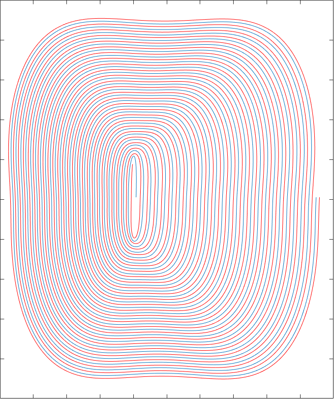
t=linspace(0, 1, 5000);

TotalTurns = 25;
CentralInitialWidth = 0.8;
Width = 50;
AsymmetricWidthCorrection = 0.035;
Width_FirstHarmonic = 4;
Width_SecondHarmonic = 1;
HorizontalDisplacement = 9;
x = (CentralInitialWidth + Width.*t).*cos(TotalTurns*2*pi.*t) .*(1 + AsymmetricWidthCorrection.*sin(TotalTurns*2*pi.*t));
x = x - Width_FirstHarmonic.*t.*cos(3*TotalTurns*2*pi.*t);
x = x - Width_SecondHarmonic.*t.*cos(5*TotalTurns*2*pi.*t);
x = x + HorizontalDisplacement.*t;

CentralInitialHeight = 20;
Height = 75;
Height_SecondHarmonic = 6;
VerticalOffset = 1;
y = (CentralInitialHeight + Height.*t).*sin(TotalTurns*2*pi.*t);
y = y - Height_SecondHarmonic.*t.*sin(5*TotalTurns*2*pi.*t);
y = y + VerticalOffset;

plot(x,y);
radius=60;
axis([-42 60 -pi/2*radius pi/2*radius]);
pbaspect([1 1 1]);

Which generates that plot:

You can play with the script by changing the values, you will understand it better than if I try to explain the purpose of each one. You can use the online version of Octave.

The parameters to define the shape, though, are not random ones. It’s the result of several iterations using my C# software to achieve the most linear gradient. There are 2 main parameters we want to optimize, which I’m going to explain using the X gradient coils as an example:

These concepts can be better understood in the following simulations.

Magnetic simulation

Having the X-Y equation which describes the electric current path, it was quite easy to integrate it to the C# simulator to generate the geometry using a 3DVector list. All the parameters of the script were also coded, so I could modify it to optimize the resultant magnetic field. I also had to add the curvature of the radius to the flat coil resulting from the previous script, since we want it projected over a cylinder. It was done by adding a sine/cosine transformation with respect to the vertical direction of the script result.

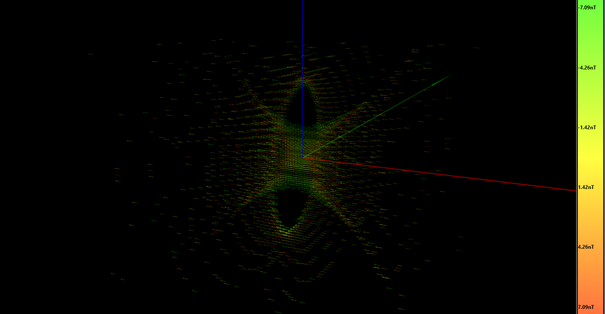
The grid is 1mm, so we have 60×60 resultant magnetic field vectors in this simulation, there is a pretty large area with good linearity and homogeneity:

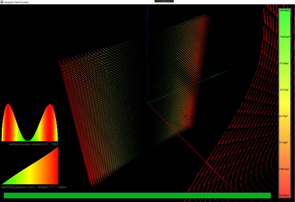
As you can observe in the simulation result, the left side vectors of the slice are pointing towards you, while the right side ones are pointing into the screen with the same magnitude but opposite direction. That’s why the gradient at the central point is zero.

The left-bottom plot shows the horizontal gradient along the X-axis (the green axis). It doesn’t perfectly fit a straight line, so the linearity could be improved, but it will be enough. We probably won’t be able to get that much resolution to worry about these tiny improvements. I have hidden 3 of the 4 coils to get better visibility, I will show the final design in a while.

The plot above the previously described is the vertical inhomogeneity along the Y-axis direction (the blue axis), but measured at the zone with the highest magnetic field (the left and right side of the slice, the same by symmetry). The difference is just 3μT with respect to the total 165μT, which is really good.

This geometry, as seen in the script, describes 4 loops of 25 turns. The simulation was run with a conductor current of 1A, which produces a maximum magnetic field of 165μT. This magnetic field will be added or subtracted to the main B0 magnetic field. That’s how we will locate the voxels along the X-axis, with a B0 of 5mT (213kHz) we will get a spin resonance of 206kHz at x=-30mm, and a resonance of 220kHz at x=30mm. Great! 🙂 An FFT of 1024 points at 213kHz has a resolution of 208Hz, which means a voxel resolution of 7·2kHz/208Hz=67 x 67 voxels. I’m just making some rude numbers, I will think about how to do this when the time comes.

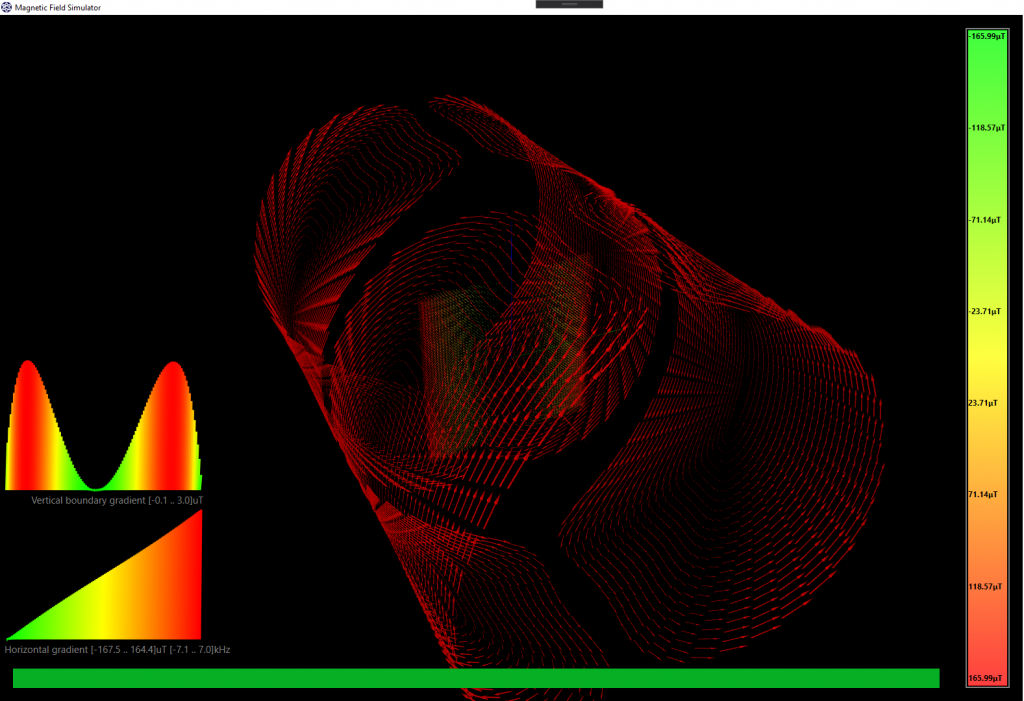
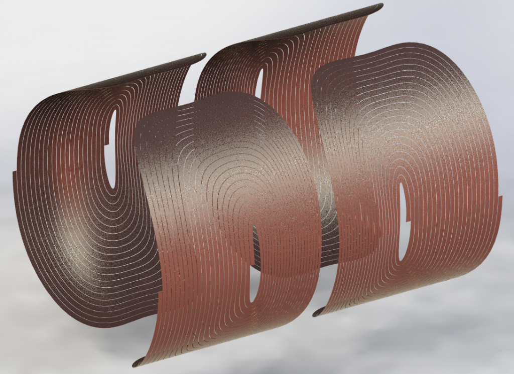
This is how the whole X-gradient geometry looks like when zoomed out:

And the render once designed in Solidworks:

A small detail that might worsen the performance is the short copper wire which will bring the current to the center of each coil. Generally speaking, all currents in this design will be transported up and down using twisted-pair cables to prevent generating magnetic interferences. But in this described case it’s not possible. I thought about doubling the number of turns by adding a second layer which would return the current to the same origin, but I don’t want to lose more time with this adding even more complexity. If I solder a short cable from the center of the coil to the extreme, and kept parallel to the Z-axis, the induced error should be quite low, and once there I will be able to solder a twisted pair cable as it should be.

The Y-gradient coils geometry is exactly the same, but with a slightly larger diameter, so that they can physically coexist without collision. Then, rotated 90 degrees along the Z-axis, so that we can generate the gradient along the Y-axis.

Physical coil implementation

The shape is hard to design by hand, that’s why I will use my laser cutter. Of course it has not enough power to cut copper, but it can cut Kapton tape. The idea is to coat a copper sheet with a layer of Kapton, and then vaporize it using laser sublimation at the zones where we want the copper to be removed. Then, add this copper sheet to a tray with etching acid which will remove that part of the copper. Some kind of PCB manufacturing process but without the substrate.

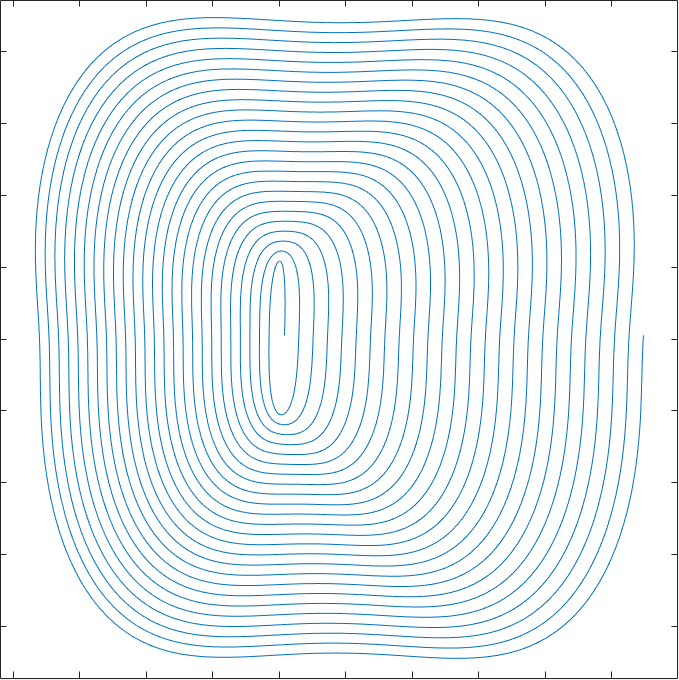
The Matlab script, as well as the C# simulation, uses the parametric equation driven curve as the path where the current flows. But we don’t want to cut by this line, we need to cut by the center of 2 consecutive lines. In this way, we ensure the current will flow by the desired path. Well, it might not be totally true, since it depends on the current density through the copper section, which in turn depends on the lowest resistance path. But anyway, using the said method is a good approximation. So I modified the parameters of Matlab script to get that second line where to cut (red line):

More results coming soon!