I’ve started writing this blog with some experiments already done. I will usually post what I’m going to do from now on, but it seems interesting to show you the results of my first attempt with permanent magnets.
It’s very tempting to have a powerless magnetic field rather than several kgs of copper dissipating heat. I knew I was trying to achieve a very unlikely achievement, but I wanted to give it a try since I already had the magnets from another project and a nice 3D printer to get the structure. A decent homogeneous magnetic field is possible on paper, but one of the main problems is the way the manufacturers magnetize the magnets. The homogeneity along the surface is not quite good, and the dispersion among the magnets is even worse.
Here I show the main idea designed and rendered using Solidworks. It consists of 26 magnets with the resultant magnetic field aligned with the X-Y plane. Each bar magnet measures 100x10x3mm, and the internal diameter of the structure, 80mm:

Here the 3D magnetic simulation, showing a slide in the YZ plane:

The central magnetic field is quite high (about 64mT) since I chose the highest grade of neodymium material for this simulation. In practice, I measured a much lower strength, who knows the characteristics of my magnets which I had there for a long time with no specs available.
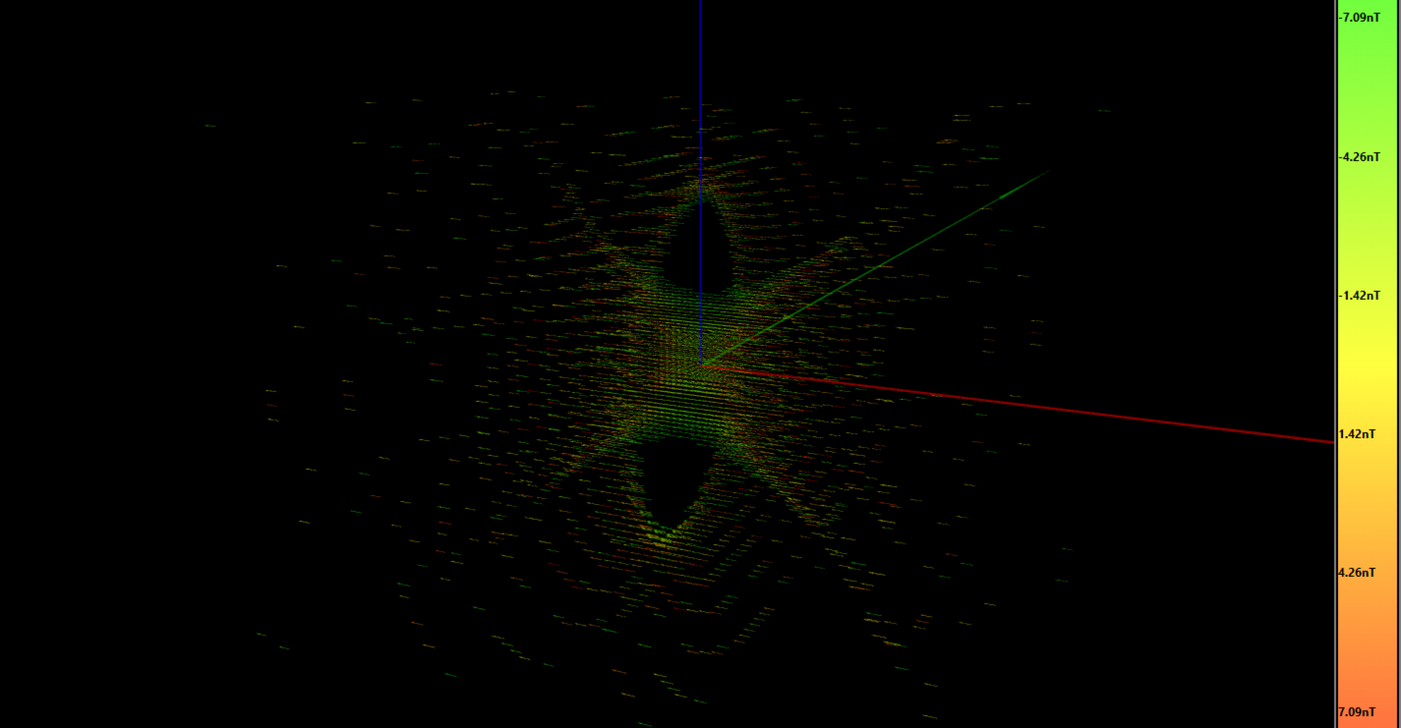
Well, simulations are pretty nice, but as already said, in the real world each magnet is different. That’s why I made a map of each magnet to select the most homogeneous ones. To do so, I attached a 3D digital hall effect sensor (TLV493D) to the head of my 3D printer. Then, using a custom software done with C# and Visual Studio, I was able to control the 3D printer through USB and sweep the sensor around the magnet. In this way I was able to get the 3D magnetic field vectors at each point. All the magnets were labeled, and the acquired data saved in a CSV file to post-process using Matlab. Here the results:
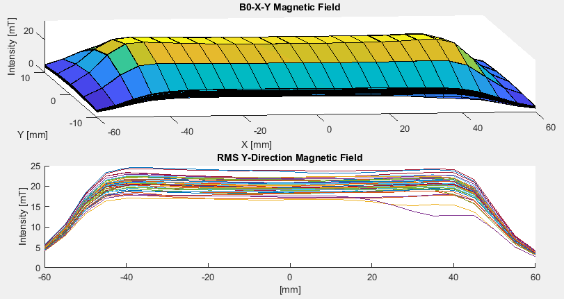
As you can see on the right side of the plot, there are at least 2 magnets that are quite inhomogeneous. From all these 44 magnets, I applied an algorithm to select the 26 most homogeneous and similar ones. I didn’t spend a lot of effort here, because I couldn’t do a miracle by just having 44 magnets available. After the selection, I processed again the data to get this plot:
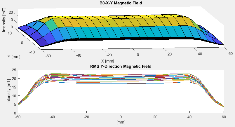
Having into account the previous magnetic field simulation, I decided to arrange the magnets within the 3D printed structure so that the strongest magnet was placed at the top/bottom and decreasing in strength in the measure I was getting closer to the center. Once assembled, I used the same previous C# software to sweep the hall effect sensor inside the structure and measure the real magnetic field. To save some time, instead of sweeping in the whole inner volume I just swept along 2 planes, here the XY plane:

The magnetic hall sensor gives 12 bit of data and a usable full scale of ±130mT. I say “usable” because if you make the math it doesn’t fit with the resolution, which is 98μT. Well, it’s a good sensor, but not good enough for our purpose. That’s why each point was highly averaged with 256 samples per point. If we suppose we have a gaussian noise, then we get 1 extra bit of resolution per x4 acquisitions, which leaves us with 12+4=16 bits of effective resolution, or what’s the same, 6.1μT. Now we are OK.
The plot data took about 1h30 to be acquired. Unfortunately, looking at the vertical axis (the magnetic strength), it’s quite obvious there would be a lot of effort to make this magnetic field homogeneous enough. Just to make me an idea, I filtered the data to know which effective volume of homogeneity we could get in the most homogeneous part. The central spot is 30.7mT, and only the data within 400ppm (12.3μT) is shown:
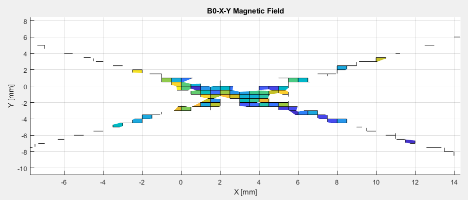
About 5x2mm of quite low homogeneous field sounds horrible, but getting a resonance of 30.7mT*42MHz/T=1.3MHz, I guess that using a small diameter glass pipe filled with water and a small diameter coil (which produces strong magnetic fields) we might have been able to measure some signal. But hey, I want much more volume! After all, I’m trying to generate an image… 😛 My conclusion, despite there are MRIs in the market which use a permanent magnet approach, is that I don’t want to waste more time with this knowing that I can get a high homogeneous field using coils and spending some time in a good design.
Stay tuned!