RF Coils

05/05/202027/05/2020

The RF coils design is also one of the main essential parts to get a decent result. By means of these coils we will excite the spins, as well as read the signal back.

First of all clarify the term “RF”, since it might cause confusion. We are not dealing with electromagnetism or radio-frequency here, just with the same kind of magnetism found in a magnet. This term is just used for historical reasons.

We already saw the main magnetic field B0 homogeneity is crucial to get some signal, but the magnetic field generated by the RF coils must also be as homogeneous as possible (not in the parts-per-million range though). The reason has to do with the flip angle, as explained below.

RF magnetic field homogeneity

As you probably know, the spins will flip its angle depending on the strength of the applied magnetic field as well as the excitation time. For example, if your spins flip 90 degrees by applying a magnetic field of B µT for t ms, you will get the same 90 degrees flip angle by applying a magnetic field of 2·B for t/2.

The whole sample is exposed to the generated magnetic field for the same amount of time, so I guess you see the problem: if for the same time t some volume in our sample is exposed to twice the magnetic field strength, instead of flipping the spins 90º they will flip 180º, and we will receive no signal at all from that volume.

Clinical MRI usually uses birdcage coils. That’s because, at 1.5T and 64MHz, the LC resonant frequency is so high that the inductance must be quite low. As low as the inductance of a single loop of wire. And it’s not helping that the geometry has to be very large to fit a human being inside, since the higher the loop area, the higher the inductance. Sometimes, the single loop is even split into smaller loops by adding capacitors in series.

Fortunately for us, we are not working at such high frequencies nor volumes. At 5mT and a resonant frequency of about 210kHz, our inductance can be much larger. Furthermore, the smaller volume also allows us to get a smaller coil, which means we can increase the number of turns. In fact, we want to have as many turns as possible in order to get as much signal as we can, as already described in Faraday’s law of induction.

Because of its well-know homogeneity, I will use a saddle coil geometry approach. Furthermore, since we are dealing with a rotating magnetic field, I will use 2 of them in quadrature, which will give us some SNR improvement. There are two factors in this SNR improvement:

1) Having more coil turns means having more signal
2) We are dealing with a non-shielded design with some external noise coupled to the coils. So the idea is to use the quadrature to get a differential signal, in this way all the common mode noise will be canceled out

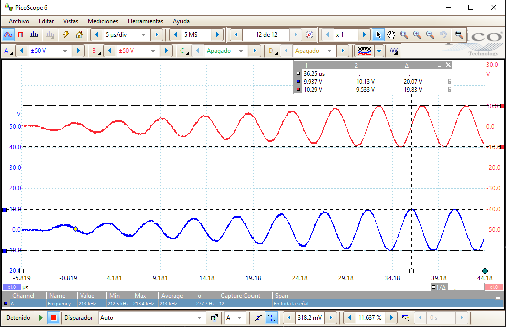
This last idea is shown here:

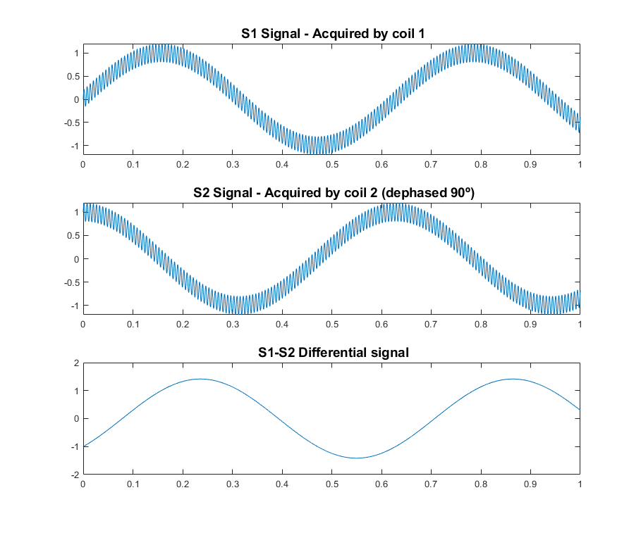
Noise reduction in differential quadrature

In both S1 and S2 signals the external noise is the same, that’s why when subtracted we get rid of it. We are not canceling out the NMR signal though, because the coils are oriented with an angle of 90º, which means we will get a sine in S1 and a cosine in S2. In other words, the resultant signal S1-S2 will be $S \cdot \sqrt{2}$ .

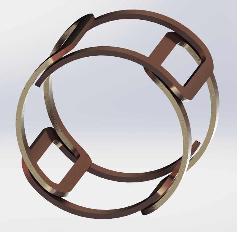
In order to totally cancel the noise out, the problem is that the external noise must be exactly coupled to all the coils. But it’s not possible with the saddle coil geometry, because it would imply to have one coil pair larger in diameter than the other one; otherwise, they would physically overlap. And having a larger coil means more area, which in turn means more external induced noise in that coil. Furthermore, it’s also important to have the same coil parameters for all of them, like inductance, series equivalent resistance, and stray capacitance. In other words, the Q factor and the self-resonant frequency. Well, everything invites us to make a design as symmetric as possible, regardless of the saddle approach. I’m going to use a modified one, like the one you can see here:

This is nice, because all the four coils are exactly the same now. The drawback is that the geometry is different, and so we have to run some more simulations to figure out what’s going on.

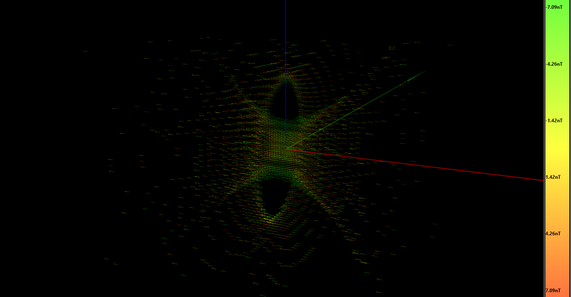
In order to achieve the best homogeneity, the saddle coil geometry is defined to have 120º between arms of the same coil with respect to the axis. To figure out which angle is the optimum one for our modified design, I’m going to sweep the saddle angle while monitoring the resultant total homogeneity using my C# program simulator. I modeled the coil geometry programmatically, because it would take me a lot of time to write another software to translate a 3D model to a list of 3D vectors used in my software. The nice thing doing it this way is that I also could program the coil geometry parameters, like the angle to sweep, which wouldn’t be possible using a “static” model approach (e.g. like importing an STL). Here I show the results:

And the same simulation looking from the side view:

It’s interesting to see how the homogeneity peaks at 142º. We have our magic angle, and it’s not 1.1º like the graphene one! 😛

Since I’ve come this far, I wanted to make one last simulation. The previous simulations show the homogeneity at 0º or 180º, but not with both coil pair working together in any angle, which is our real case when we get the rotating magnetic field. That’s what is shown in that last simulation:

At the bottom-left side you can see how the homogeneity fluctuates over time. The magnetic field is only constant at the central point, so, for a real and accurate result, I should have integrated each voxel with the exposed magnetic field over one entire turn. That’s how I would know the total energy received by each water molecule and so the real flip angle. Despite this, I didn’t want to waste more time here since I see quite good results in the central slice. Furthermore, I wouldn’t know how to improve this design further, I’ve done my best at this point.

I haven’t mention it, but I’ve dimensioned the coils to have a diameter as small as possible, but containing as much as B0 homogeneous magnetic field as possible. That’s how I pretend to get a maximum filling factor.

Mechanical design

Once the coil geometry is clear, I’ve designed the custom coil former, which I 3D printed. Here you can see a 3D render animation:

This design makes the coil winding process quite hard and slow, because of its closed design which forces me to wind it like a toroid inductor. Furthermore, after winding one coil, I saw it was difficult to get a good symmetry, because of the half-open concept which keeps one sector more squeezed than the other. That’s why I designed a more sophisticated system, where each coil can be wound individually, and then fixed altogether using nylon screws:

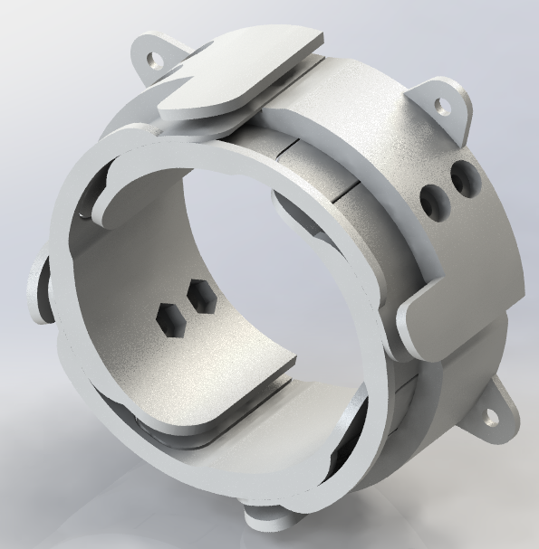
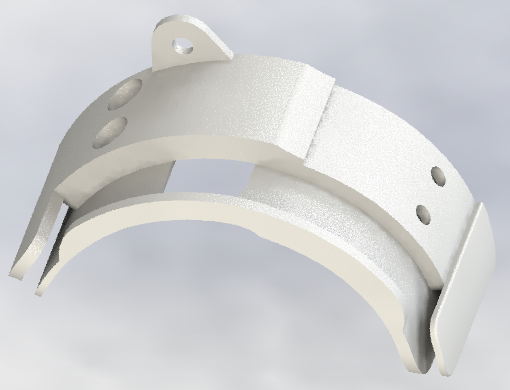
Which is the composition of 4 exactly equal and symmetric coil formers like this one:

Electrical parameters

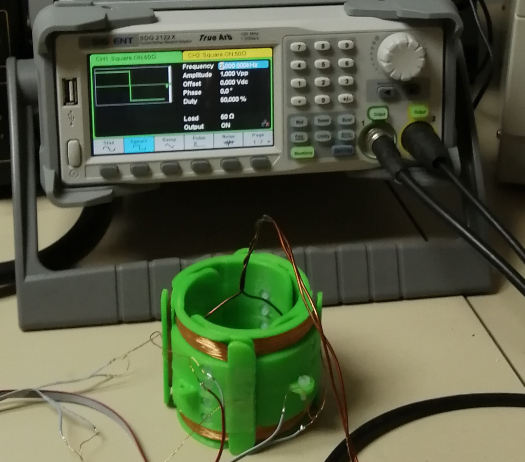
I wound a single coil to get a rough idea of the coil’s main parameters. The thing is that I could calculate the resultant inductance and series resistance using the Solidworks plugin, which gives you that information taking into account the coil geometry, number of turns, and wire diameter. But I couldn’t get the stray capacitance, which I have no means/knowledge to calculate it. Furthermore, it’s very dependent on the way the coil is wound: it’s not the same to have some overall initial coil section overlapped with some final section, than to have a perfect wound vertical section for each turn around the whole coil. After winding one coil I saw it’s hard to get that perfect vertical section, because the radial force toward the center in the curved plane makes that the wires spread on the surface. That’s why in my redesign I’ve given a bit more space in the axial direction. Now the coil should fit much better without overlapping at the final turns, and now I clearly see it’s almost impossible to calculate the stray capacitance.

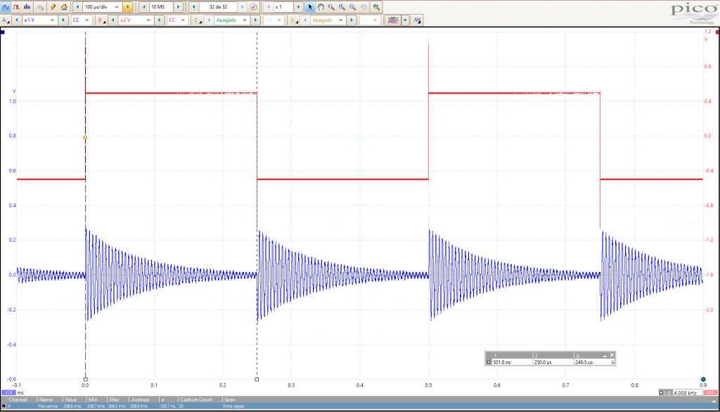
That stray capacitance is a very important factor because, together with the coil inductance, it produces a self-resonant frequency. If that self-resonance is close to the nuclear magnetic resonance, we will have no room for the input impedance of our signal amplifier. The worst-case would be that the self-resonance became lower than the NMR frequency, in this case we could get no measure at all.

Summarizing: given a maximum copper volume defined for our coil former, this design is a trade-off between self-capacitance and series resistance while trying to keep the maximum number of turns.

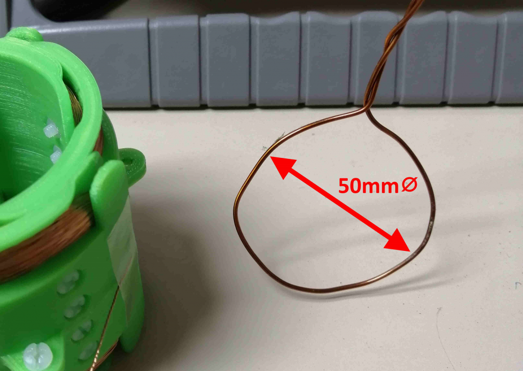
I used 110 turns of 2x 0.2mmØ joined together. The thing is I needed 0.3mm copper wire but I didn’t have any reel available. Just mention that at 210kHz the skin effect for a 0.3mmØ wire begins to be perceptible, but not enough to justify the use of Litz wire. I used my NanoVNA device to get the parameters:

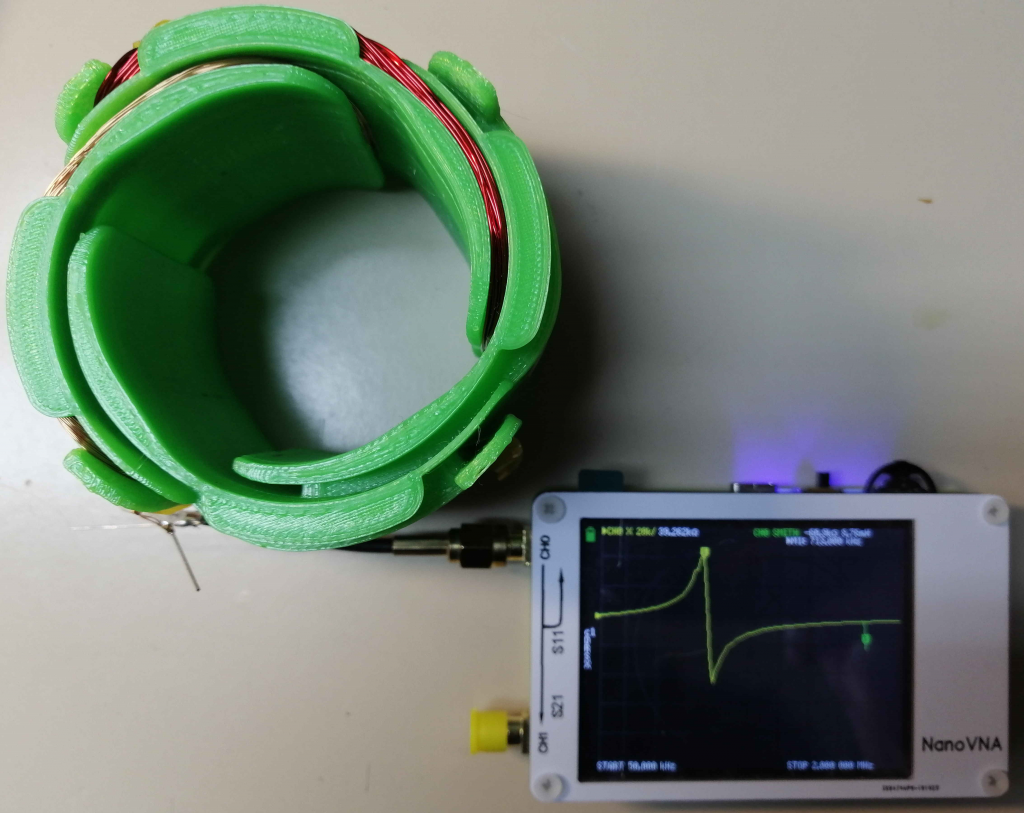
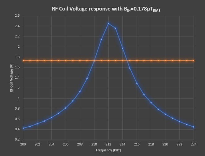
Which in this setup are:

Resonant frequency: 715kHz
Inductance: 1.5mH
Stray capacitance: 33pF
Series resistance: 7ohm

This is not the exact final design, but it is telling me I’m on the right way. Given the previous parameters, the Q factor at 210kHz is 283, quite good! 🙂 Putting it all together, my conclusion is that I will use few more turns when winding the 0.3mmØ copper wire in my final coil former. Adding more turns will increase the Q factor because the inductance increases quadratically with the number of turns while the resistance only linearly. But the self-resonant frequency will be lowered at a much faster rate as well, since apart from the inductance, also the stray capacitance increases. As far as we keep the self-resonant frequency with a good margin above the desired NMR frequency, we should wind as many turns as possible to maximize the NMR signal.

Another useful parameter derived from the above data is the $A_L$ of our air core coil former, which is of about $1.24\cdot10^{-7}H/N^{2}$ . So I can calculate the inductance for any number of turns, e.g. for 130 turns, $L=1.24\cdot10^{-7}\cdot130^{2}=2.1mH$ . In this last case, the resistance would increase from 7Ω to 8.7Ω, but the Q factor would increase from 283 to 318. I have no idea about the stray capacitance in this new case, but supposing no capacitance variation, we would have a self-resonant frequency of about 600kHz (which will be lower due to the real higher stray-capacitance). I guess I will try with about 150 turns if the coil former allows me to fit all of them.

More results coming soon!

27/05/202027/05/2020

Assembly and Testing

In the following video, I show the 3D printing process of the RF coil formers, the result of the windings in 2 pieces, and the final assembly by joining the 4 pieces using non-magnetic nylon screws.

To observe the rotating magnetic field effect, I use a neodymium magnet diametrically polarized. From both coil pairs assembled in quadrature, a sinusoidal current is applied to the first one (using a function generator), and the same current dephased 90º is applied at the second pair, as can be observed in the screen.

The 300mHz generates a complete magnet turn approximately every 3 seconds, although, in the MRI, we will use 213kHz at 5mT.

Since motors don’t care about homogeneity, it probably is the most homogeneous magnetic field motor in the world right now 😛

31/05/202031/05/2020

Testing the RF coils

Since I still don’t have the quadrature differential amplifier assembled, I’ve tested a single coil pair (2 opposite side coils connected in series) using the function generator and the oscilloscope. Here the steps:

The coil pair is connected to the CH1 of the oscilloscope. The oscilloscope probe was set to 10x to reduce the stray capacitance, which now decreased to 13pF
A single turn copper wire loop with a diameter of 50mm was placed in the center of the RF coil structure. It was axially rotated until finding the maximum signal. In this position, if turned 90º, we would receive no signal (it would be received by the other coil pair)
Then, I’ve connected the output of the function generator directly to the previous copper wire loop. The output impedance of the function generator has a standard 50Ω impedance, and the copper wire loop, a short circuit. So, configuring the output with 1V square wave at 2kHz, the current to the single turn coil is 1V/50Ω=20mA. In this way, I’m generating a pulsed magnetic field, and thus I can see the output response of the coil pair

The single copper wire loop:

The setup:

And finally, the output resonating signal:

I’ve added an external 100pF capacitor to tune to the desired 210kHz, which added to the probe capacitance of 13pF means a total of 113pF.

I calculated the generated magnetic field by using the single wire loop equation:

$\vec{B}=\frac{\mu_{0}I}{2R}\hat{j}=\frac{4\pi 10^{-7}0.02}{2\cdot 0.025}\hat{j}=0.5\mu T$

Here in Catalunya, we have an earth magnetic field of around 45μT, which means I’m generating a pulse about 90 times smaller. Despite this, we can see an output response of about 0.5V_PP. Not bad!

Q Factor

The theoretical values for the Q factor given the 2 measured coil parameters are:

Coil pair 1: 4.44mH and 16.8ohm. It means a Q Factor of 349 @ 210kHz
Coil pair 2: 4.48mH and 16.8ohm. It means a Q Factor of 351 @ 210kHz

One way to measure the real Q is by using the resonating decaying signal. It consists of counting how many cycles it takes to reach half the initial voltage, and then, multiply that value by 4.53. Taken the previous acquisition, we see a Q=13·4.53=58, about 6 times lower than theoretically expected. In other words, the effective AC resistance became about 100Ω. The reason is the high frequency losses.

For such a “low” frequency and the wire diameter used, the skin effect is not a problem. But the proximity effect really is, where the magnetic field generated by the current flowing by the wire itself induces currents to the other adjacent wires.

For an unloaded RF coil (meaning there is no water sample), the Q factor usually goes from 50 to 600, while a loaded RF ranges from 10 to 100. So, we are in the worst-case range. The number of turns increases the proximity effect losses, although it also increases the sensitivity.

One might think that the highest the Q factor the better, because it is the ratio between the stored energy and the energy lost per cycle. But that’s not actually true, some NMR labs even intentionally decrease the Q by adding a series resistor. The thing is that the highest the Q factor, the sharper the frequency response, and the lowest the bandwidth. And we need some bandwidth to acquire the MRI signal when we apply the gradient magnetic fields.

The bandwidth can directly be calculated from the Q factor, but I wanted to measure it to make sure. So I swept a constant current sinusoidal signal through the single wire loop, and measured the RMS voltage at the output of the LC resonator. Here the result:

The orange trace shows the -3dB level, defined as the bandwidth threshold

In this case, there is no surprise and the theoretical value corresponds with the real one. The Q factor is defined as:

$Q=\frac{f_r}{BW}=\frac{212kHz}{4kHz}=53$

I don’t really know the NMR implications about not having a so high Q factor, but what I do know is that 4kHz of bandwidth is a perfect span for the gradient magnetic fields, as already seen in the next gradient section.

Finally, from the above plot we can directly get the sensitivity:

$Sensitivity=\frac{2.45V_{RMS}}{0.178\mu T_{RMS}}=13.78V/\mu T \, @ \, 212kHz$

08/02/202108/02/2021

Measurement of the RF pulse signal

The initial design with the PCB planar transformer gave quite bad results in terms of signal distortion. That’s why I decided to use one pulse transformer per quadrature channel.

This transformer is a 1:1:1 (meaning it has 3 independent and equal coils). I use the first coil to apply the signal, and connecting the other two in series I get an output voltage 2 times higher than the input.

The signal applied to the trasformer comes from an operational amplifier working at 24V, with a maximum output voltage span of about 2V to 22V. I use 2 operational amplifiers to transform the single DAC output voltage (from 0 to 2.5V) to a differential voltage of ±20V. With the extra 2x gain of the transformer, we get a total output voltage of 80V_PP which can be directly applied to the RF coils.

Final desing with two VTX-110-006 pulse transformers

Mesurement of the static RF coil magnetic field

To calculate the flip angle given by the RF pulse, we first must know the magnetic field generated by the RF coils (which using the common nomenclature, we will call B1). So I used a digital magnetometer. I know it’s not the most accurate way to do it, but it’s a good starting point. Once I get some NMR signal, we will be able to play with the flip angle to find the optimum value.

The magnetometer was placed in the middle of the RF coil. I used a STM32 eval board to get the magnetometer data using I2C, and send it to the PC using a USB VCP. Then I applied some different currents to the coil to get this table:

I_DC [A]	Mag [µT]
0.00637	21
0.0152	50
0.0298	98
0.0595	195
0.0714	233

Now we just need to know the impedance of the coil at the NMR frequency. It’s important to measure it instead of just calculating it, because we also want to have into account the high frequency loses (like the proximity effect one). So I used a 216Ω shunt resistor to measure the current with the oscilloscope, and I applied 8.6V_PP with the function generator. A simple V/I division gives an impedance of 6435Ω @ 213kHz.

Flip angle and flip time

The flip angle just depends on the time we apply the pulse and the magnitude of the applied magnetic field (B1). Here the equation:

$PulseTime=\frac{DesiredAngle}{360 \cdot LarmorFrequency \cdot B1}$

Knowing that we can generate up to 80V_PP, we can get the current of the coil from the previous calculated parameters:

$MaxCoilCurrent=\frac{80V_{PP}}{6435\Omega}=12.4mA_{PP}$

Now, from the tendency line equation found out in the previous plot, we can find out the B1:

$B1=3260.7 \cdot 12.4mA_{PP}+0.5388=41\mu T_{PP}=20.5\mu T_{P}$

We now will use the peak magnitude instead of the peak to peak. It is clear why when we apply the common trick of switching to the rotating frame of reference, so that we now rotate with the nucleus and see a static magnetic field. The quadrature system with a sine/cosine signal will make that the nucleus sees a static and constant magnetic field with a magnitude equal to the peak value.

Note that to flip the spin angle to 90 degrees we are talking of only 20μT! This result was quite shocking to me, since it’s about half the earth magnetic field! I didn’t expect that…

Now we have all we need to calculate the flip time to get a 90 degree flip angle:

$PulseTime=\frac{90}{360 \cdot 42.58MHz/T \cdot 20.5\mu T} = 285\mu s$

This time is equivalent to:

$213kHz \cdot 285\mu s=61 sinusoidal\ cycles$

Quadrature signal

Here I show the oscilloscope capture of the 2 signals which are applied to the RF coils. They are generated with the internal DAC peripheral of the microcontroller, a DAC configured in dual mode (both channels updated at the same time) to send the signal to each channel. It’s actually the same signal, but shifted 90º to give the quadrature feature.

The signal shape is first calculated using a “for” loop, and stored in a RAM array. Then, using a timer, each data in the RAM array is transferred to the DAC using a DMA. The resultant signal is very smooth, since I’m running the DAC at 5MSPS to generate the 213kHz. All this process is already generated inside the microcontroller, but I have some programming work to do to control everything from the computer.