It’s been a while from my last post. I started a new small project to improve the cooling water system of my cutter laser device. The original 40W CO2 laser tube died, and I had to replace it. After some research I found out that the original system (water tank + pump) was not enough, since the water temperature must be regulated between 15 and 20 degrees, and the room temperature can reach to be as high as 30 degrees in summer. That’s why I used 2 water pumps with 2 different circuits, 4 peltiers (12V @ 15A), some temperature sensors, velocity controlled fans using PWM, heatsinks, a water radiator, a custom controller board to control everything, and all of crazy stuff. The thing is it is now working like a charm, and all the methacrylate pieces to build the MRI structure have already been cut.
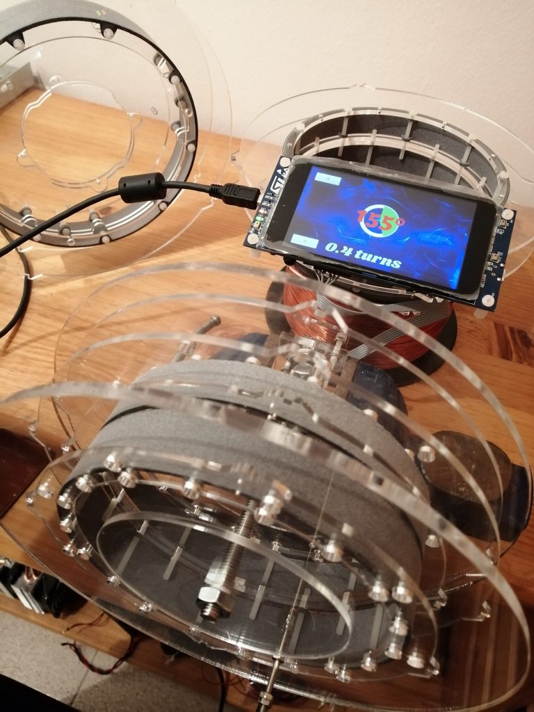
I also did another small project with a digital magnetic angular sensor + ST eval board with a capacitive TFT display and TouchGFX, so that I can start winding the coils without loosing a single loop. Here a photo of the setup:
Once I get all the coils winded and assembled to the main structure, I’ll come back with more news 🙂
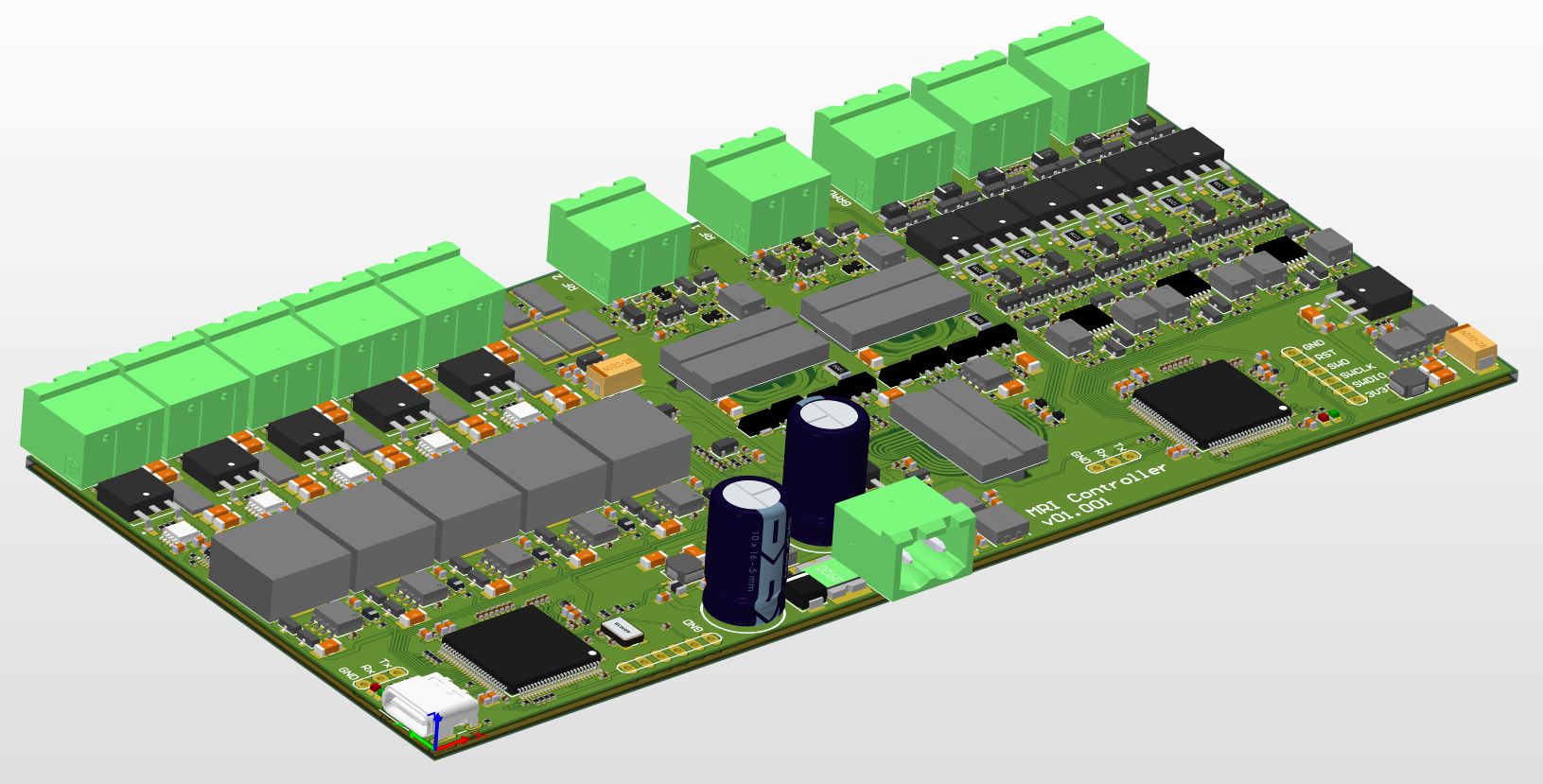
It took me about 2 weeks of work in my free time, but the PCB is finally finished! The main features:
5 independent channels of DCDC + linear current source to drive the 5 coils which generate the main B0 magnetic field. One 16-bit dual DAC per channel is used to configure the current setpoint, as well as generating an ultra-high precision 2.5V reference with low temperature drift and very low noise. Apart from using this reference for the current sources, the reference is spread through the board to be used as the main reference for the microcontroller’s ADCs, the signal amplifiers, the NTC sensor and the gradient coil drivers
2 independent drivers to generate the quadrature rotating magnetic field (RF field), as well as 2 amplifiers and all the logic to switch from transmitter to receiver. A third differential amplifier with some extra gain is used to remove the common mode noise and to acquire the NMR signal
3 independent drivers to generate the X, Y and Z gradient magnetic fields. The Z gradient field might not finally be used, since the simulations showed an homogeneity zone of just 1.5cm in the Z direction, but the driver will be there just in case
Two microcontrollers are used (STM32H7 family). The master is used to communicate with the computer through USB (USB 2.0 over a USB C connector) and to send commands to the slave. It also controls the PWMs of the 5 drivers to generate the B0 magnetic field, and to control each linear current source using each DAC (through SPI). It also measures the temperature using a NTC, thermally coupled to all the shunt resistors, and compensates the current setpoint when the shunt resistors temperature changes according to the temperature coefficient of each resistor, which was chosen as low as possible (100ppm/ºC).
The slave microcontroller is the one that performs the main MRI tasks. It generates both RF signals (the main and the 90º shifted one) using both internal DACs + DMA. It also controls the gradient magnetic field timings, and the integrated 16-bit ADC @ more than 5MSPS is used to capture the 210kHz signal.
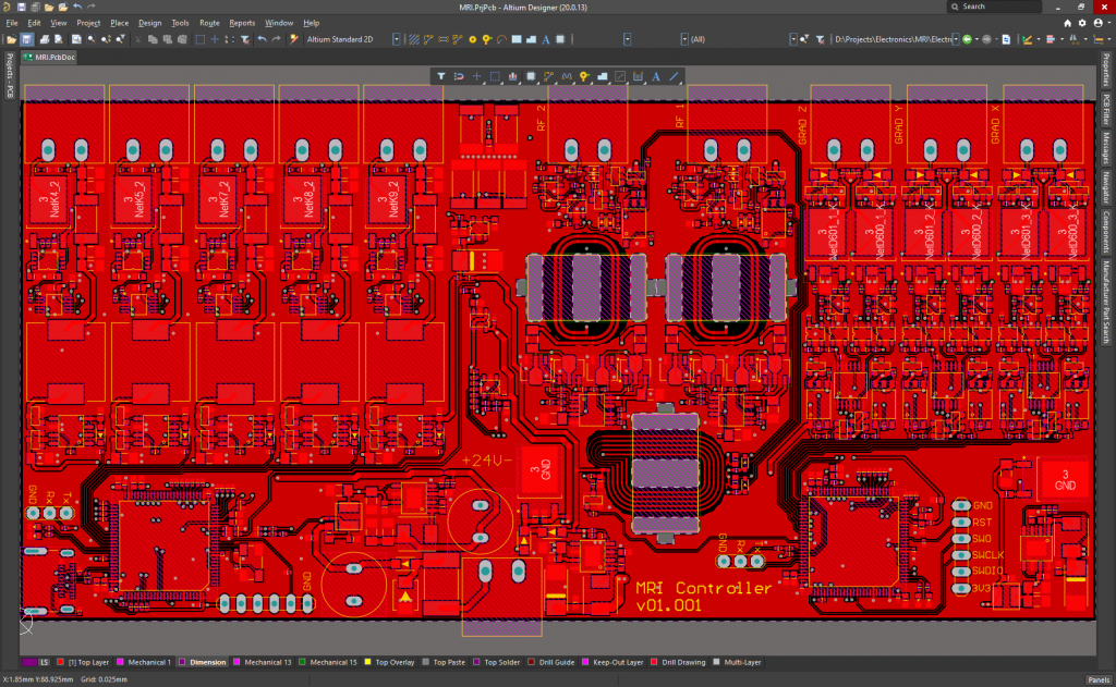
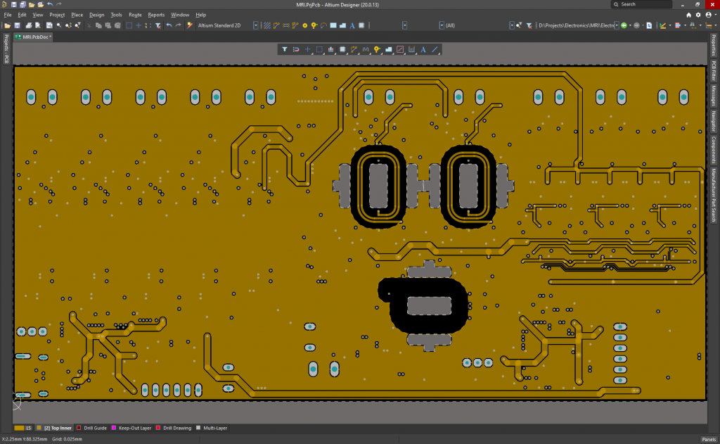
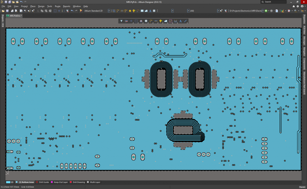
PCB Layers:
Top Layer
Top-Internal Layer
Bottom-Internal Layer
Bottom Layer
It is powered at 24V, although the microcontrollers can run and be programmed using the 5V of the USB C connector when plugged to the PC. It measures 165.2mmx80mm, and it has been ordered to Eurocircuits today.
I will assemble it next week, I’ll post the results soon!
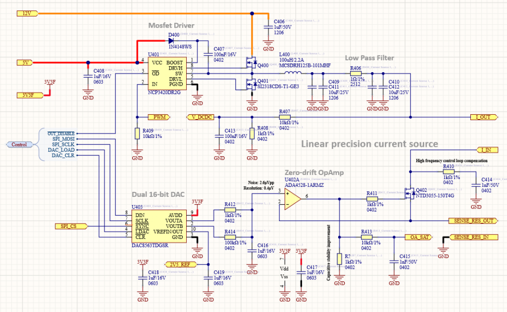
Working hard on the electronic schematics these days! I’m done with the main B0 current source, finally with less than 3µVPP of noise from 0.1 to 10Hz and 0.4µV of resolution. The voltage-to-current conversion will depend on the shunt resistor, where the worst case is when using a 0R47: the noise and resolution will be of 6µAPP and 0.8µA. I need that much resolution to get the required magnetic field trimming.
I’m also using an NTC close to the current sense resistors, thermally coupled among them and chosen with the same size and PPM/ºC, to compensate by firmware the resistor variations due to self-heating.
I’m using a DC/DC controlled by the microcontroller to adjust the voltage in the MOSFET drain, and let it work in the linear region. I need the DC/DC because too much voltage across the MOSFET implies too much dissipated power. The main microcontroller will initially perform a calibration:
1. Set a current of let’s say 100mA using the 16-bit DAC
2. Start increasing the duty cycle of the PWM to rise the I_OUT voltage
3. While increasing, keep checking the OA_SAT pin. Right now it will be 3.3V because the small I_OUT voltage makes few current to flow through the coil, and the MOSFET will be in the saturation region. But when the OA_SAT pin becomes <3.3V will mean that we just left the saturation region, so we just need to increase about 0.5V more to give the MOSFET some margin to work properly in the ohmic region without dissipating too much power
A better way would be to connect the I_IN voltage to an ADC input, but it should have to be done through an operational amplifier with low bias current, or the shunt resistor would measure the sum of both currents and the precision would be lost.
A 100µH seems a pretty high value for the DC/DC, but we want the ripple current to be as low as possible. With a so large inductor, we don’t need large capacitors, but what is really important is that they have a low ESR, since that’s the main source of ripple noise. In this case, it’s MUCH better to have a total of 40µF using ceramic capacitors than 470µF using an electrolytic one.
Finally, about the high frequency control loop compensation network. It was added there because we are using a current source to control the current of a VERY large inductor (the one which generates the main B0 magnetic field). Without that network, the operational amplifier would be unstable and it would oscillate.
Today I’ve just been playing with my software to render this 3D animation of the magnetic field generated by a Helmholtz coil. The objective was to observe how the magnetic homogeneity varies with respect to the distance between coils.
As you can see, we find the maximum homogeneity when the distance between coils equals the radius (70mm). The total central magnetic field is also decreasing as the coils spread apart. In each of the 300 simulations to generate this animation, the central magnetic field is calculated and plotted to the left graph, and then only the 3D vectors fitting the 100ppm volume are shown. The homogeneity is also plotted below the central magnetic field graph, and the maximum variability shown in the right color scale in nT.
I’ve started writing this blog with some experiments already done. I will usually post what I’m going to do from now on, but it seems interesting to show you the results of my first attempt with permanent magnets.
It’s very tempting to have a powerless magnetic field rather than several kgs of copper dissipating heat. I knew I was trying to achieve a very unlikely achievement, but I wanted to give it a try since I already had the magnets from another project and a nice 3D printer to get the structure. A decent homogeneous magnetic field is possible on paper, but one of the main problems is the way the manufacturers magnetize the magnets. The homogeneity along the surface is not quite good, and the dispersion among the magnets is even worse.
Here I show the main idea designed and rendered using Solidworks. It consists of 26 magnets with the resultant magnetic field aligned with the X-Y plane. Each bar magnet measures 100x10x3mm, and the internal diameter of the structure, 80mm:
Bar magnet circular array to get a high central homogeneous magnetic field
Here the 3D magnetic simulation, showing a slide in the YZ plane:
Magnetic field simulation in the central plane
The central magnetic field is quite high (about 64mT) since I chose the highest grade of neodymium material for this simulation. In practice, I measured a much lower strength, who knows the characteristics of my magnets which I had there for a long time with no specs available.
Well, simulations are pretty nice, but as already said, in the real world each magnet is different. That’s why I made a map of each magnet to select the most homogeneous ones. To do so, I attached a 3D digital hall effect sensor (TLV493D) to the head of my 3D printer. Then, using a custom software done with C# and Visual Studio, I was able to control the 3D printer through USB and sweep the sensor around the magnet. In this way I was able to get the 3D magnetic field vectors at each point. All the magnets were labeled, and the acquired data saved in a CSV file to post-process using Matlab. Here the results:
Measured magnetic field of all the 44magnets I had available
As you can see on the right side of the plot, there are at least 2 magnets that are quite inhomogeneous. From all these 44 magnets, I applied an algorithm to select the 26 most homogeneous and similar ones. I didn’t spend a lot of effort here, because I couldn’t do a miracle by just having 44 magnets available. After the selection, I processed again the data to get this plot:
Magnetic field measurement of the 26 most homogeneous ones
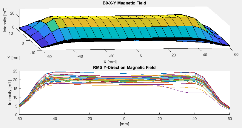
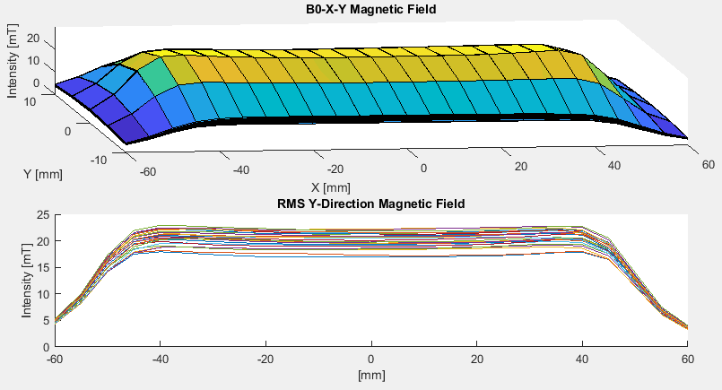
Having into account the previous magnetic field simulation, I decided to arrange the magnets within the 3D printed structure so that the strongest magnet was placed at the top/bottom and decreasing in strength in the measure I was getting closer to the center. Once assembled, I used the same previous C# software to sweep the hall effect sensor inside the structure and measure the real magnetic field. To save some time, instead of sweeping in the whole inner volume I just swept along 2 planes, here the XY plane:
XY Magnetic field inside the permanent magnet structure
The magnetic hall sensor gives 12 bit of data and a usable full scale of ±130mT. I say “usable” because if you make the math it doesn’t fit with the resolution, which is 98μT. Well, it’s a good sensor, but not good enough for our purpose. That’s why each point was highly averaged with 256 samples per point. If we suppose we have a gaussian noise, then we get 1 extra bit of resolution per x4 acquisitions, which leaves us with 12+4=16 bits of effective resolution, or what’s the same, 6.1μT. Now we are OK.
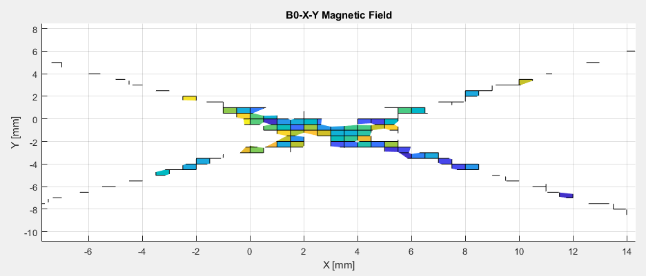
The plot data took about 1h30 to be acquired. Unfortunately, looking at the vertical axis (the magnetic strength), it’s quite obvious there would be a lot of effort to make this magnetic field homogeneous enough. Just to make me an idea, I filtered the data to know which effective volume of homogeneity we could get in the most homogeneous part. The central spot is 30.7mT, and only the data within 400ppm (12.3μT) is shown:
Central homogeneity for the permanent magnet structure – 400ppm
About 5x2mm of quite low homogeneous field sounds horrible, but getting a resonance of 30.7mT*42MHz/T=1.3MHz, I guess that using a small diameter glass pipe filled with water and a small diameter coil (which produces strong magnetic fields) we might have been able to measure some signal. But hey, I want much more volume! After all, I’m trying to generate an image… 😛 My conclusion, despite there are MRIs in the market which use a permanent magnet approach, is that I don’t want to waste more time with this knowing that I can get a high homogeneous field using coils and spending some time in a good design.