Bernat Albet – Page 2 – Electronic Projects

07/08/202013/08/2020

PCB finished and ordered

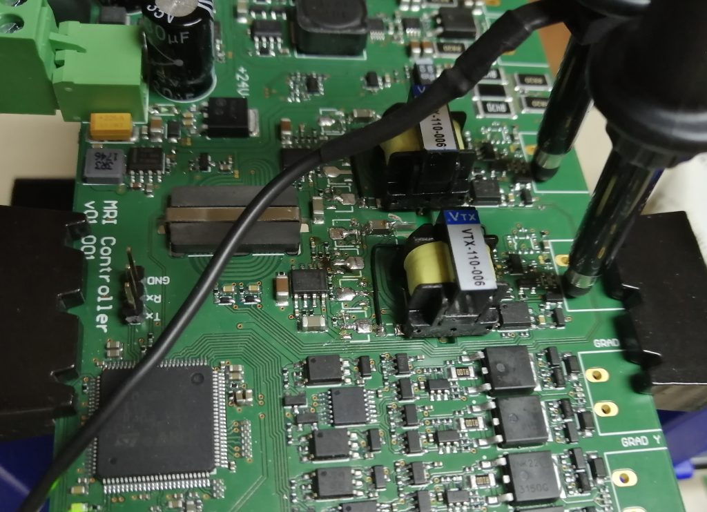
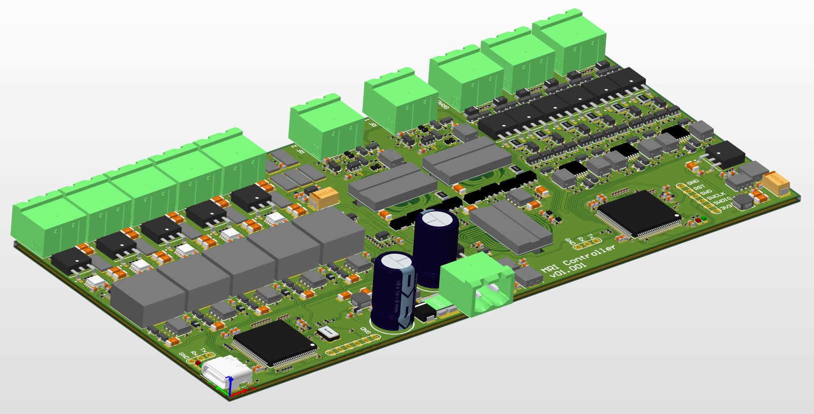
It took me about 2 weeks of work in my free time, but the PCB is finally finished! The main features:

5 independent channels of DCDC + linear current source to drive the 5 coils which generate the main B0 magnetic field. One 16-bit dual DAC per channel is used to configure the current setpoint, as well as generating an ultra-high precision 2.5V reference with low temperature drift and very low noise. Apart from using this reference for the current sources, the reference is spread through the board to be used as the main reference for the microcontroller’s ADCs, the signal amplifiers, the NTC sensor and the gradient coil drivers
2 independent drivers to generate the quadrature rotating magnetic field (RF field), as well as 2 amplifiers and all the logic to switch from transmitter to receiver. A third differential amplifier with some extra gain is used to remove the common mode noise and to acquire the NMR signal
3 independent drivers to generate the X, Y and Z gradient magnetic fields. The Z gradient field might not finally be used, since the simulations showed an homogeneity zone of just 1.5cm in the Z direction, but the driver will be there just in case

Two microcontrollers are used (STM32H7 family). The master is used to communicate with the computer through USB (USB 2.0 over a USB C connector) and to send commands to the slave. It also controls the PWMs of the 5 drivers to generate the B0 magnetic field, and to control each linear current source using each DAC (through SPI). It also measures the temperature using a NTC, thermally coupled to all the shunt resistors, and compensates the current setpoint when the shunt resistors temperature changes according to the temperature coefficient of each resistor, which was chosen as low as possible (100ppm/ºC).

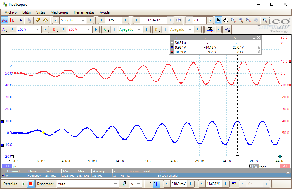
The slave microcontroller is the one that performs the main MRI tasks. It generates both RF signals (the main and the 90º shifted one) using both internal DACs + DMA. It also controls the gradient magnetic field timings, and the integrated 16-bit ADC @ more than 5MSPS is used to capture the 210kHz signal.

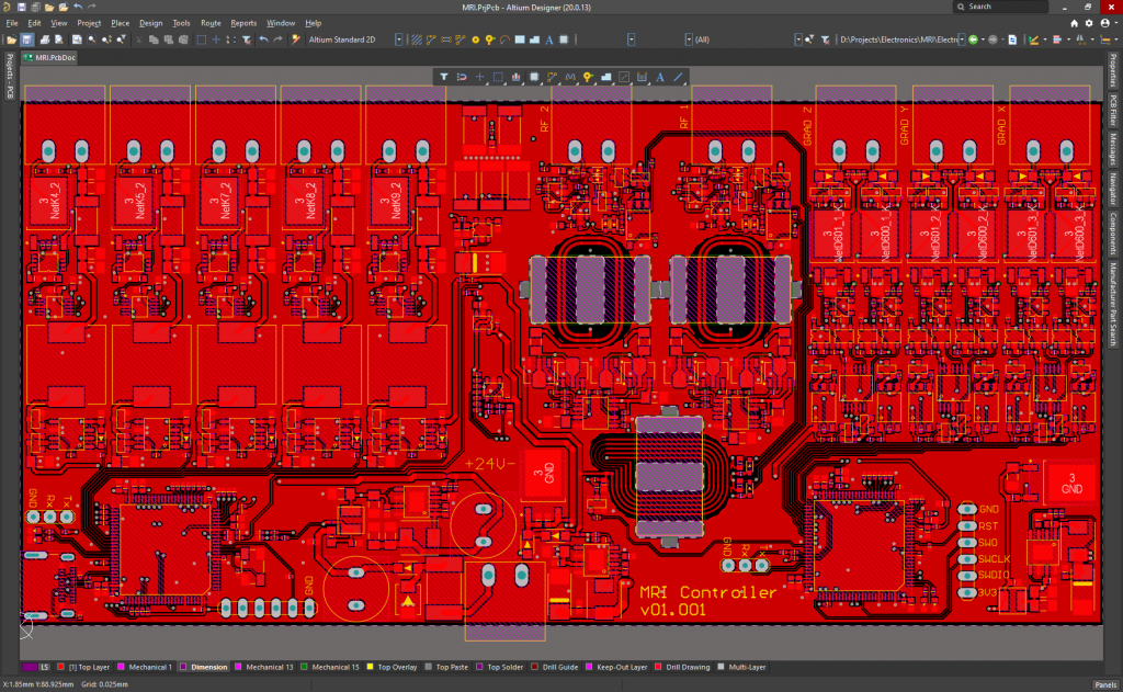
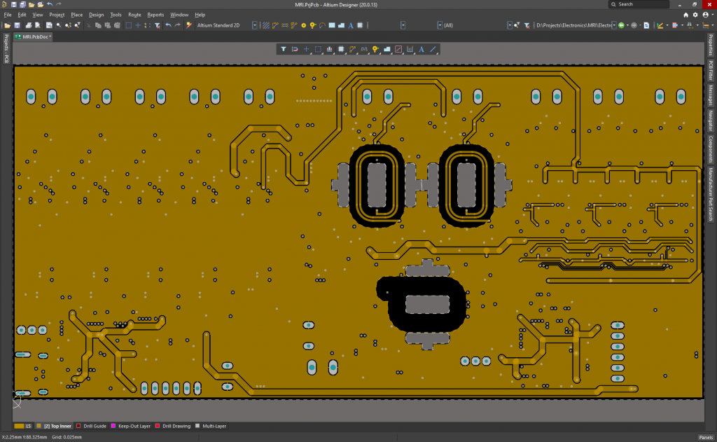
PCB Layers:

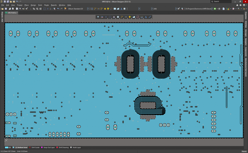
It is powered at 24V, although the microcontrollers can run and be programmed using the 5V of the USB C connector when plugged to the PC. It measures 165.2mmx80mm, and it has been ordered to Eurocircuits today.

I will assemble it next week, I’ll post the results soon!

02/10/202002/10/2020

Project update

It’s been a while from my last post. I started a new small project to improve the cooling water system of my cutter laser device. The original 40W CO2 laser tube died, and I had to replace it. After some research I found out that the original system (water tank + pump) was not enough, since the water temperature must be regulated between 15 and 20 degrees, and the room temperature can reach to be as high as 30 degrees in summer. That’s why I used 2 water pumps with 2 different circuits, 4 peltiers (12V @ 15A), some temperature sensors, velocity controlled fans using PWM, heatsinks, a water radiator, a custom controller board to control everything, and all of crazy stuff. The thing is it is now working like a charm, and all the methacrylate pieces to build the MRI structure have already been cut.

I also did another small project with a digital magnetic angular sensor + ST eval board with a capacitive TFT display and TouchGFX, so that I can start winding the coils without loosing a single loop. Here a photo of the setup:

Once I get all the coils winded and assembled to the main structure, I’ll come back with more news 🙂

08/02/202108/02/2021

Measurement of the RF pulse signal

The initial design with the PCB planar transformer gave quite bad results in terms of signal distortion. That’s why I decided to use one pulse transformer per quadrature channel.

This transformer is a 1:1:1 (meaning it has 3 independent and equal coils). I use the first coil to apply the signal, and connecting the other two in series I get an output voltage 2 times higher than the input.

The signal applied to the trasformer comes from an operational amplifier working at 24V, with a maximum output voltage span of about 2V to 22V. I use 2 operational amplifiers to transform the single DAC output voltage (from 0 to 2.5V) to a differential voltage of ±20V. With the extra 2x gain of the transformer, we get a total output voltage of 80V_PP which can be directly applied to the RF coils.

Final desing with two VTX-110-006 pulse transformers

Mesurement of the static RF coil magnetic field

To calculate the flip angle given by the RF pulse, we first must know the magnetic field generated by the RF coils (which using the common nomenclature, we will call B1). So I used a digital magnetometer. I know it’s not the most accurate way to do it, but it’s a good starting point. Once I get some NMR signal, we will be able to play with the flip angle to find the optimum value.

The magnetometer was placed in the middle of the RF coil. I used a STM32 eval board to get the magnetometer data using I2C, and send it to the PC using a USB VCP. Then I applied some different currents to the coil to get this table:

I_DC [A]	Mag [µT]
0.00637	21
0.0152	50
0.0298	98
0.0595	195
0.0714	233

Now we just need to know the impedance of the coil at the NMR frequency. It’s important to measure it instead of just calculating it, because we also want to have into account the high frequency loses (like the proximity effect one). So I used a 216Ω shunt resistor to measure the current with the oscilloscope, and I applied 8.6V_PP with the function generator. A simple V/I division gives an impedance of 6435Ω @ 213kHz.

Flip angle and flip time

The flip angle just depends on the time we apply the pulse and the magnitude of the applied magnetic field (B1). Here the equation:

$PulseTime=\frac{DesiredAngle}{360 \cdot LarmorFrequency \cdot B1}$

Knowing that we can generate up to 80V_PP, we can get the current of the coil from the previous calculated parameters:

$MaxCoilCurrent=\frac{80V_{PP}}{6435\Omega}=12.4mA_{PP}$

Now, from the tendency line equation found out in the previous plot, we can find out the B1:

$B1=3260.7 \cdot 12.4mA_{PP}+0.5388=41\mu T_{PP}=20.5\mu T_{P}$

We now will use the peak magnitude instead of the peak to peak. It is clear why when we apply the common trick of switching to the rotating frame of reference, so that we now rotate with the nucleus and see a static magnetic field. The quadrature system with a sine/cosine signal will make that the nucleus sees a static and constant magnetic field with a magnitude equal to the peak value.

Note that to flip the spin angle to 90 degrees we are talking of only 20μT! This result was quite shocking to me, since it’s about half the earth magnetic field! I didn’t expect that…

Now we have all we need to calculate the flip time to get a 90 degree flip angle:

$PulseTime=\frac{90}{360 \cdot 42.58MHz/T \cdot 20.5\mu T} = 285\mu s$

This time is equivalent to:

$213kHz \cdot 285\mu s=61 sinusoidal\ cycles$

Quadrature signal

Here I show the oscilloscope capture of the 2 signals which are applied to the RF coils. They are generated with the internal DAC peripheral of the microcontroller, a DAC configured in dual mode (both channels updated at the same time) to send the signal to each channel. It’s actually the same signal, but shifted 90º to give the quadrature feature.

The signal shape is first calculated using a “for” loop, and stored in a RAM array. Then, using a timer, each data in the RAM array is transferred to the DAC using a DMA. The resultant signal is very smooth, since I’m running the DAC at 5MSPS to generate the 213kHz. All this process is already generated inside the microcontroller, but I have some programming work to do to control everything from the computer.