Magnetic field B0

This is one of the most important and complex parts in the design, and it happens to be the first one to deal with. That’s because all the rest of the design constraints will be based on the result of this one. Three parameters are the most important ones:

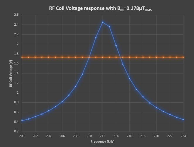
1) Magnetic field strength: Through the gyromagnetic ratio of the hydrogen (42.58MHz/T), the magnitude of this main magnetic field will directly give us the resonant frequency of our spins (also called the Larmor frequency), and so, a great part of the electronics design. Furthermore, for higher magnetic field strengths, not only the frequency is higher, but the amplitude as well. After the simulations, I can anticipate that the coils will generate 5mT. At such a low field, we are speaking of 5mT*42MHz/T= 210kHz. Very low compared with a real MRI with 1.5T and 64MHz… Let’s see what we can do with that

2) Magnetic homogeneity: It’s one of the most important issues, and where I spent most of my time with simulations. If you imagine the whole water sample as the sum of small water volumes, having a low homogeneous magnetic field means that each of them will see a different magnetic field strength, and so, they will resonate at a slightly different frequency. It means that after the generation of the RF pulse to synchronize all the spins, the phase among the spins will gradually be lost, as well as the signal to measure. In a high strength magnetic field this wouldn’t be so dramatic, since the resonant frequency would be much higher, and for the same inhomogeneity and amount of time, we would have many more cycles to acquire the signal. But that’s not our case, complexity is growing!

3) Effective volume: Unfortunately, there is no way to make a perfect straight magnetic field line in the real world. So, we can define the effective volume as the volume where the magnetic field is constant enough to get the required small spin dephasing which allows us to measure the signal. As I will explain later, I found a method to achieve a magnetic field lower than 10ppm over several cm3 of volume (at least in theory). The effective volume is important because it will give us the constraints for the RF coil geometry. In order to get a high filling factor and as much SNR as possible, it should cover as much effective volume as possible, and at the same time, cover the maximum water sample volume as possible.

In order to generate high homogeneous magnetic fields, the way to go is using coils. Maybe in a few years we will have available some nice graphene room temperature superconducting wires hehe But until then, we have no other choice but to deal with copper.

There are some standard geometries already known to get highly homogeneous magnetic fields, like the Helmholtz coils. But for our purpose, I want a coil which performs a better job. The first thing I did was programming a Visual Studio software (C# is my preferred high-level language) to simulate magnetic fields given any conductor shape based on the Biot-Savart law. The main idea was to use my custom software to design the main structure, but the 3D calculations were so CPU demanding that I had to find another approach. Once the CPU calculations are done, WPF is great, since it uses the GPU to render the graphics. Now I just use this software to validate and observe the final result, to design the main structure I finally used Matlab.

I use a Solidworks plugin to simulate magnetic fields, but just to get a rough idea. We are dealing with ridiculously tiny scales here. For example, 10ppm of 5mT results in a magnetic field variability of 50nT, 1200 times weaker than the earth’s magnetic field. At this point, these kinds of software which use a solid mesh approach are not precise enough. Furthermore, you can’t process the data results in a custom manner.

Matlab script

As well as I did in my custom C# software, I implemented the discrete Biot-Savart law to calculate the final resultant magnetic field. Despite this, they were coded a bit different:

In C#, I calculate all the 3D magnetic vectors in each volume point, having into account all the defined objects carrying some current. So, it is the most generic version of the Biot-Savart equation

In Matlab, I coded a specific case of the generic equation, the case where we have loops of wires. So, a first step calculates the magnetic field along the central X-axis given the X_0 position, the radius, and the current I. Then, we iterate for each defined loop wire (with different X_0 and radius) to integrate the final resultant magnetic field. But just along the X-axis. That’s why I will use the C# software to visualize the resultant 3D field of the entire structure once it is defined using this script

That’s how it works:

function [x,B,R,P,len,kg] = CalculateMagneticField(Winding, Radius_mm, I, wireDiameter_mm)

Winding: A matrix of [N, X] elements. Each matrix value can be 0 or 1, depending on the coil being populated with copper wire or not. The X position multiplied by wireDiameter_mm/2 gives the distance along the wires:

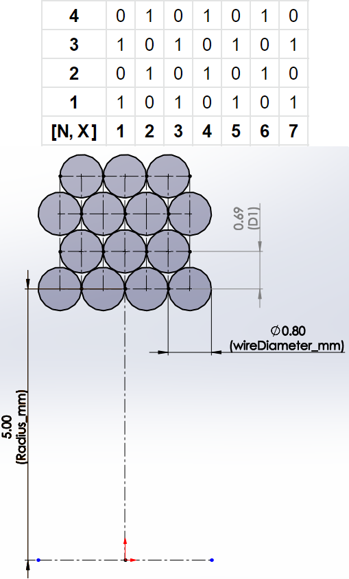
Radius_mm: The radius of the first layer from the central axis. The rest of the radii are automatically calculated having into account we are using round-shaped wires. The image above shows how the vertical distance is lower than the wire diameter. Simple trigonometry shows the fitting factor is wireDiameter_mm·cos(30). Despite this, since the coil is wound back and forth and the spiral will change the direction in each new layer, the radius will vary from wireDiameter_mm·cos(30) to wireDiameter_mm, depending on the turn angle. In fact, it will have 2 maximum and 2 minimum peaks per turn, fluctuating at each 90º. It means that, if perfectly wound, it would create an elliptical shape if lots of turns were required. But we live in a non-ideal world, and the coil former width will not mathematically be as designed. So each time we reach the end of the coil former and the spiral changes in direction, the angle will randomly dephase a bit. These cumulative errors make us a favor, and so I will use the average as an effective fitting factor: wireDiameter\_mm \cdot \frac{1+cos(30)}{2}
I: The current of the whole winding
wireDiameter_mm: Just comment that I used a fitting factor outside this function, so, instead of using 0.8mm for a 0.8mm diameter wire, I will use 0.86mm for imperfections when winding

Then, it returns:

x: A vector, where each element contains the position of each calculated magnetic field B, with 0mm located at half the vector. Its length equals the X size of the winding matrix
B: A vector with the resultant magnetic field, corresponding with the previous distances
R: Total resistance of the resultant coil
P: Total power dissipated by the coil, given the current I and the previous calculated R
len: Total copper wire length to wind this coil
kg: The total copper weight

After coding this function, I tried to use a solver to maximize the homogeneity, but it’s a complex function to solve. It couldn’t converge, or converge at non maximized solution (I tried with the simple Helmholtz coil). So, I just did it myself. I programmed a second script which will call the previous one to act as a tool to make this coil design process easier for me. I empirically started with 1 central winding of X turns and N layers per turn. Then, modifying X and N, as well as the radius, I could observe how the final resulting magnetic field changed along the central X-axis. At this point I was watching myself as an IA network training myself hahaha Here I show this script in action:

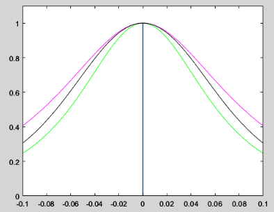
In green, I show the magnetic field for a 1 single loop wire. In pink, a 100 turns coil organized in 100 layers (multi-layer, thin coil). And finally in black, also 100 turns but organized in 1 single layer (single layer, wide coil). As you can see I show the unitary magnetic field, of course a 100 layer coil generates a much higher magnetic field than a single layer. But the scale can be changed by changing the current, on the other hand the shape of the magnetic field can not be adjusted and just depends on the geometry.

To get the most homogeneous magnetic field, we need to get a straight line at the center, where we now see a curved shape. As you can see, we need to form a straight line adding curves.

Here I configured the script to plot a Helmholtz coil. I set a radius of 70mm and, as the geometry requires, a separation between coils of 35mm (radius/2). Each coil formed by just 3 wires of 1mm of diameter:

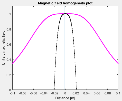
The 2 vertical blue lines show the zone where the homogeneity is lower than 10ppm of the central magnetic field. In this case, 3.5mm. The pink line is the total unitary result, and the black line is the vertical unitary zoom of the pink line (amplified about 5000 times). In this way, if I separate a bit both coils, we can observe the effect in the black line but not in the pink one:

Separating the coil 2mm from each other, the homogeneity zone is decreased to 2.5mm. The black line shows the effect of the coil separation, which is weakest now at the center.

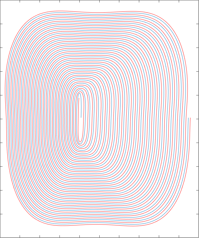
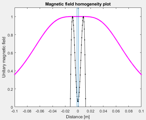
Seeing the above image, I thought the way to make a more homogeneous magnetic field was separating even more both coils, and adding an extra central coil, where the central peak would add to the central notch and make it more straight. After that step, I saw that adding a second couple of coils (a total of 5 now) would improve a bit more the homogeneity. Despite this, adding more coils was not effective for the size I was dealing with. The peaks are too broad and overlap too much with each other. Here I plot the final result after lots of iterations:

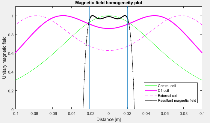
The black line now, apart from the zoom, is also the sum of all the 3 magnetic fields, generated by the central coil, and the 2 pairs of extra coils. I used the black line to know where the magnetic field was too weak or too strong, then I could adjust the adjacent turn wires and current to make the center as flat as possible. With this solution, the homogeneous magnetic field zone increases up to 34mm, with 4ppm from the central 5mT. This means we have a magnetic field of 5mT ± 10nT! Great 🙂

I could even get a flatter response, it is a trade-off which reduces the homogeneous zone.

The way to calculate the number of turns and geometry was iterating, knowing the effects that have adding layers or making the coil wider, as seen before in the first script example. I could also play with the currents to increase the magnetic field of each pair of coils when I didn’t want to increase the number of turns (but having into account that I want the same dissipated power in each coil). After some time playing with the script, I started to see some patterns and what to do to make the lobes flatter. The results of the script:

Central Magnetic field: 5.001 mT
Larmor freq: 212.9443 kHz
Total Power: 8.407W
Homogeneous space: 34mm
Copper weigth: 6.7249kg

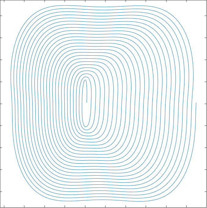
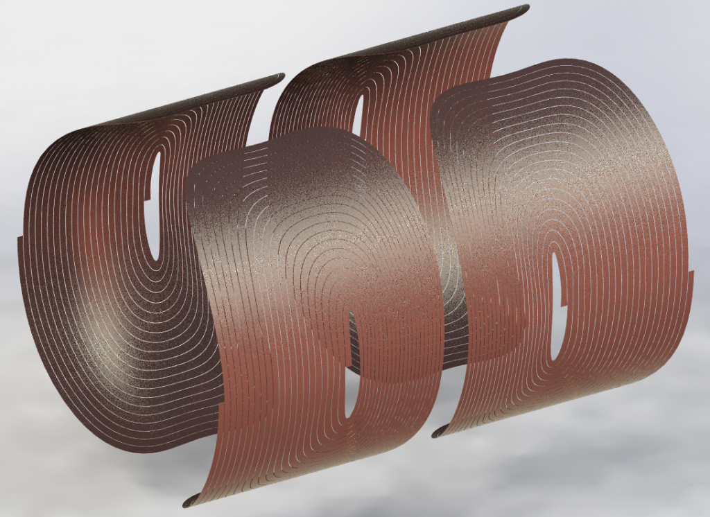
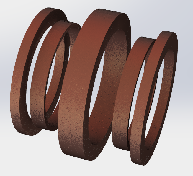
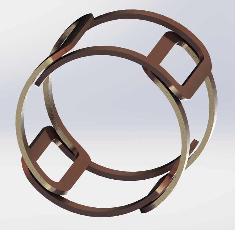
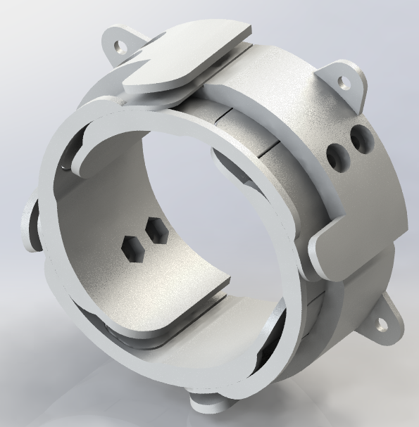
Furthermore, the script writes a text file with the dimensions of the coils, in a format that Solidworks can understand using the equation editor. In this way, just executing the script, Solidworks can update the shape of the final result, which you can see here:

The results for each individual coil, with a copper wire diameter of 0.86mm:

Central Coil:
CC Current= 303.5134 mA
CC Coil Turns= 1125
CC Total R= 20.8815 ohm
CC Wire Length= 641.1368 m
CC Coil Weight= 3.0337 kg
CC Voltage= 6.3378 V
CC Power= 1.9236 W

C1 Coils:
Displacement from center=±54.12mm
C1 Current= 628.7246 mA
C1 Coil Turns (1/2)= 204
C1 Total R (1/2)= 3.0428 ohm
C1 Wire Length (1/2)= 93.4263 m
C1 Coil Weight (1/2)= 0.4421 kg
C1 Voltage (1/2)= 1.9131 V
C1 Power (1/2)= 1.2028 W

External coils:
Displacement from center=±79.54mm
CE Current= 459.3984 mA
CE Coil Turns (1/2)= 585
CE Total R (1/2)= 9.6607 ohm
CE Wire Length (1/2)= 296.6185 m
CE Coil Weight (1/2)= 1.4035 kg
CE Voltage (1/2)= 4.4381 V
CE Power (1/2)= 2.0389 W

T2* due to the homogeneity

I’ve said that 4ppm is good enough, but I want to demonstrate it in numbers. At 5mT, the Larmour frequency is 212.9kHz. Since that frequency is proportional to the magnetic field, we can calculate the 4ppm over the frequency, which gives 212.9kHz±0.85Hz. In other words, the most dephased spins will take about 1.2 seconds to dephase 360º. I will use 90º of dephasing for this calculation since it’s a good approach to the time constant 𝜏 (usually 67%), and so our T2* would be of 90º/360·1.2s= 300ms. This is good! A T2 for water is usually in the order of 1.5 seconds. It has no sense to make more accurate numbers here since this will differ in reality, too many factors in real life, this was a rough approximation.

Of course, I have my concerns about achieving 4ppm, which are theoretical values given a perfect geometry. Furthermore, all these calculations were done with a relative permeability of copper = 1, the same as air, but in reality copper is a bit diamagnetic. And with “a bit” I mean \mu/\mu_0=0.999994. The error is in the order of some few ppm, so I guess we will be able to shim it using tiny current variations in each coil, the thing is the calculations would be too complex having into account this effect.

An advantage of this design is that I will use 5 different current sources, one for each coil, to shim the magnetic field. I will only be able to shim it in the Z direction though.

The earth’s magnetic field will also add up to our generated B_0. We are talking about 1.2% of our 5mT. As seen in the Terranova device, they use shimming to improve the earth’s magnetic field. In our case, we will also have the 1.2% of the earth’s magnetic field inhomogeneities, which will fall into the sub-ppm region having into account we also have a smaller volume (if we don’t have any magnetic object close enough, of course). Despite this, the effect we might observe is a small shift in the expected final resonance, for example 212.52kHz instead of 210kHz (1.2%), but it can be adjusted with the shimming currents easily. Apart from this, I don’t know of any other external magnetic field which can affect us, just small misalignments between the 5 coils. I’m thinking about using some kind of hardware fine trimming for moving the external coils in small amounts, but some simulations showed that an error smaller than 1mm can be fixed adjusting the currents in each coil wire.

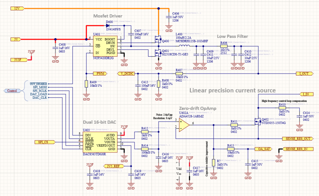
Another factor of a MAJOR consideration, even supposing we achieve a perfect and ideal copper winding structure, is the resolution of our current sources. The numbers are frightening and another challenge to overcome. As an example, our central coil runs at about 0.3A. If we want to be able to shim the magnetic field in 1ppm, we are talking about controlling 0.3μA! That’s insane… Some years ago I designed an EEG, so I can tell you that here we are dealing in the same order of magnitude than the signals generated by the brain on the surface of the scalp, with the aggravating that our full-scale is WAY larger.

One thing in our favor is that these huge coils with so many turns have a large inductance, which is good to keep the currents constant even using a DCDC. But the DC stability is what seems more difficult to solve. That’s because the spin-echo only works if the magnetic field is constant from the 90º pulse to the TE time, otherwise, the frequencies varies a bit and the 180º effect doesn’t compensate the inhomogeneities. The water itself is proportional to the resonant frequency, so we could use this fact as feedback to adjust the overall coils current, but this can only be done at the time we acquired the signal, not between pulses.

Lots of things will have to be taken into account, like the very-small resistance changes of our shunt resistors due to the temperature heating effect (which might be huge when talking about μA), the problem of voltage offsets drift in our amplifiers, ADC non-linearities, etc. I will show the numbers when I write that section.

Magnetic field simulation using the custom C# software

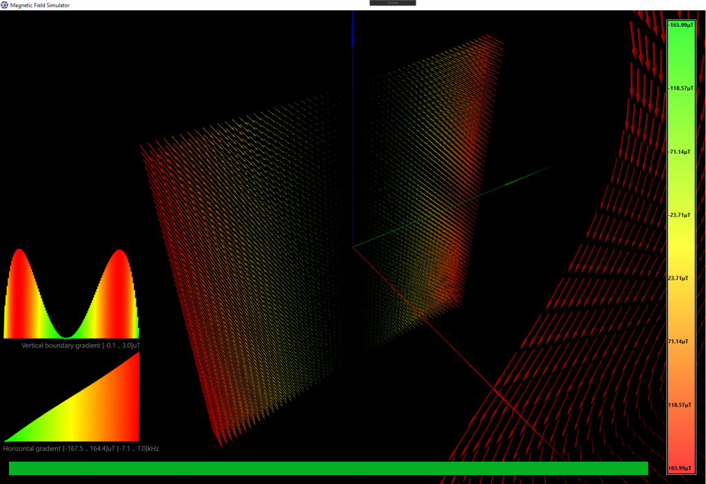
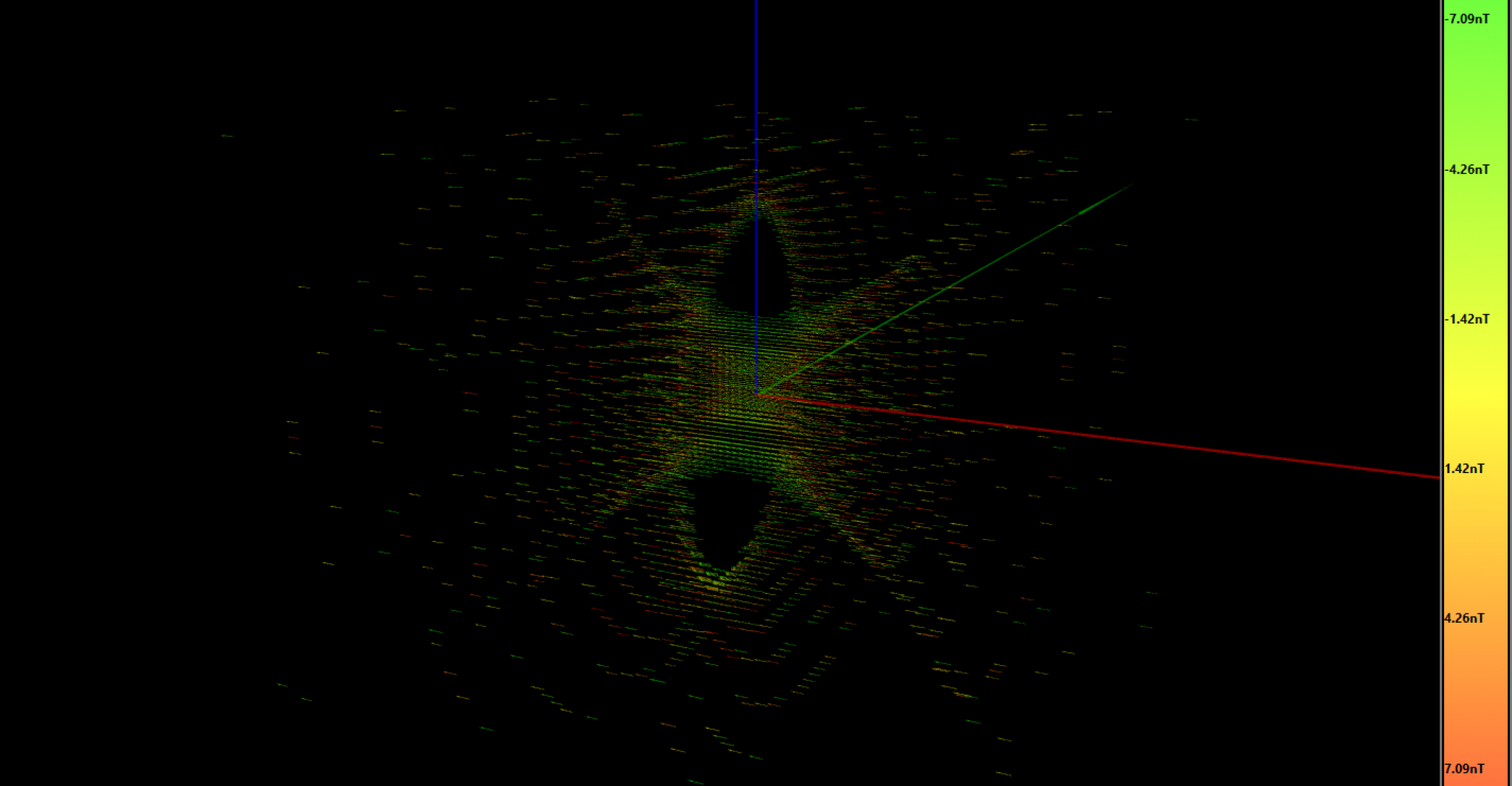
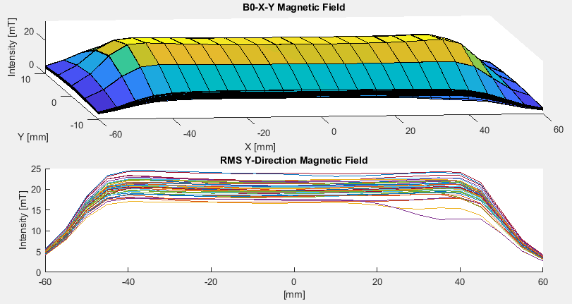
I coded the geometry and the current for each coil, according to the results of the Matlab script. As already said, we just calculate the magnetic field along the X-axis, so here we will see the final 3D result and the homogeneity volume. I made a video because it’s worth seeing in movement. The first simulation is for a 1mm grid, only showing the vectors falling inside the 2ppm region:

The vector count is 3341, which means that in this volume we have at least 3341mm³ (we can call them voxels) of 2ppm in magnetic homogeneity.

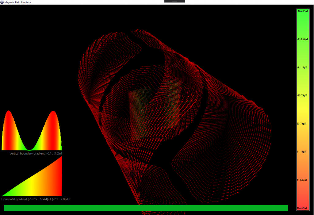
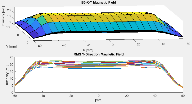
This second simulation is the same, increasing the homogeneity to 4ppm. The number of voxels now increased to 7267 (equivalent to 7.3cm³):

I haven’t uploaded the 6ppm video because it was quite similar to the previous one, but the zone increased up to 10171 voxels (10.2cm³). Not bad! Although I was expecting a higher volume.

The simulator took about 10 minutes to perform all the calculations, even using strategies in C# to run the code in all the 8 cores of my computer.

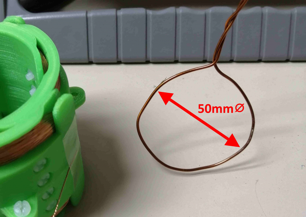
This information is very useful because now we can adjust the geometry of the RF coil to maximize the filling factor. We have about 4cm of diameter and 1.5cm of length where we have our most homogeneous magnetic field to get a useful image.

Finally, just as a matter of comparison, I designed a Helmholtz coil using the same technique. The Helmholtz coil has a separation between coils equal to the radius, but it’s only true when you have a few copper turns. As already seen before, adding more turns (in height or width) widens the shape of the resultant magnetic field, so the separation has to be adjusted to achieve the flattest curve at the center. I tried the results to be as much similar as possible to my design:

C1 Coil
Displacement=40.18mm
C1 Current= 630.1560 mA
C1 Coil Turns (1/2)= 706
C1 Total R (1/2)= 10.9933 ohm
C1 Wire Length (1/2)= 337.5348 m
C1 Coil Weight (1/2)= 1.5971 kg
C1 Voltage (1/2)= 6.9275 V
C1 Power (1/2)= 4.3654 W

Central Magnetic field: 5.084 mT
Larmor freq: 216.4761 kHz
Total Power: 8.7308W
Homogeneous space: 5.3309mm
Copper weigth: 3.2137kg

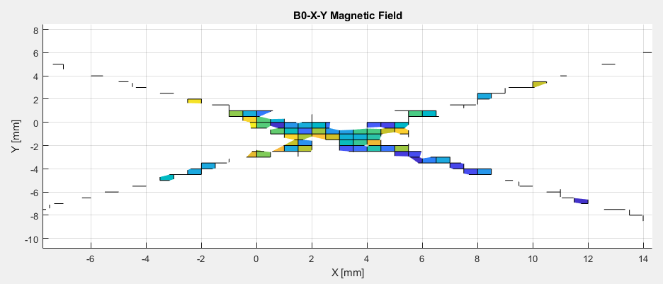
After running the simulation, only 591 elements were found (0.6cm³) in the 6ppm volume, in comparison with the 10.2cm³ we could achieve with our 5-coil approach. For its design I tried to achieve the same dissipated power (8.7W vs 8.4W) to get the same magnetic field. As you can see, I need about 2.1 times the total copper volume, but I achieve 17 times more homogeneity than in the Helmholtz coil, so I guess the extra copper is worth to be paid! 😛

For the video, instead of running the previously designed Helmholtz structure, I run the simplest Helmholtz form using only 2 thin conductors. The coils also separated 35mm instead of 40.2mm found to be better in the previous specific case. In this most generic case, only 291 volume elements (0.29cm³) were found in the 6ppm range. It has sense because the shape of the magnetic field is sharper than in wider coils:

As you could notice, in all these simulations it’s only shown half of the windings. It’s done on purpose to prevent the background coil to visually interfere, but of course in reality the copper will be there. That’s it for today!

Stay tuned!

MRI Project

This is the main project which motivated me to create this website. Be aware this is an ongoing project, which I’m going to publish the results in the measure I move forward.

As you can imagine, I will start trying to develop a low field NMR device. Despite this, since I need to design a PCB, I will do it thinking in the electronics to manage all the gradient magnetic fields.

Magnetic field homogeneity using a permanent magnet approach

I’ve started writing this blog with some experiments already done. I will usually post what I’m going to do from now on, but it seems interesting to show you the results of my first attempt with permanent magnets.

It’s very tempting to have a powerless magnetic field rather than several kgs of copper dissipating heat. I knew I was trying to achieve a very unlikely achievement, but I wanted to give it a try since I already had the magnets from another project and a nice 3D printer to get the structure. A decent homogeneous magnetic field is possible on paper, but one of the main problems is the way the manufacturers magnetize the magnets. The homogeneity along the surface is not quite good, and the dispersion among the magnets is even worse.

Here I show the main idea designed and rendered using Solidworks. It consists of 26 magnets with the resultant magnetic field aligned with the X-Y plane. Each bar magnet measures 100x10x3mm, and the internal diameter of the structure, 80mm:

Bar magnet structure to get a central homogeneous magnetic field
Bar magnet circular array to get a high central homogeneous magnetic field

Here the 3D magnetic simulation, showing a slide in the YZ plane:

Magnetic field simulation in the central plane

The central magnetic field is quite high (about 64mT) since I chose the highest grade of neodymium material for this simulation. In practice, I measured a much lower strength, who knows the characteristics of my magnets which I had there for a long time with no specs available.

Well, simulations are pretty nice, but as already said, in the real world each magnet is different. That’s why I made a map of each magnet to select the most homogeneous ones. To do so, I attached a 3D digital hall effect sensor (TLV493D) to the head of my 3D printer. Then, using a custom software done with C# and Visual Studio, I was able to control the 3D printer through USB and sweep the sensor around the magnet. In this way I was able to get the 3D magnetic field vectors at each point. All the magnets were labeled, and the acquired data saved in a CSV file to post-process using Matlab. Here the results:

Magnetic field measurement of 44 neodymium bar magnets
Measured magnetic field of all the 44 magnets I had available

As you can see on the right side of the plot, there are at least 2 magnets that are quite inhomogeneous. From all these 44 magnets, I applied an algorithm to select the 26 most homogeneous and similar ones. I didn’t spend a lot of effort here, because I couldn’t do a miracle by just having 44 magnets available. After the selection, I processed again the data to get this plot:

Magnetic field measurement of the 26 most homogeneous ones

Having into account the previous magnetic field simulation, I decided to arrange the magnets within the 3D printed structure so that the strongest magnet was placed at the top/bottom and decreasing in strength in the measure I was getting closer to the center. Once assembled, I used the same previous C# software to sweep the hall effect sensor inside the structure and measure the real magnetic field. To save some time, instead of sweeping in the whole inner volume I just swept along 2 planes, here the XY plane:

XY Magnetic field inside the permanent magnet structure

The magnetic hall sensor gives 12 bit of data and a usable full scale of ±130mT. I say “usable” because if you make the math it doesn’t fit with the resolution, which is 98μT. Well, it’s a good sensor, but not good enough for our purpose. That’s why each point was highly averaged with 256 samples per point. If we suppose we have a gaussian noise, then we get 1 extra bit of resolution per x4 acquisitions, which leaves us with 12+4=16 bits of effective resolution, or what’s the same, 6.1μT. Now we are OK.

The plot data took about 1h30 to be acquired. Unfortunately, looking at the vertical axis (the magnetic strength), it’s quite obvious there would be a lot of effort to make this magnetic field homogeneous enough. Just to make me an idea, I filtered the data to know which effective volume of homogeneity we could get in the most homogeneous part. The central spot is 30.7mT, and only the data within 400ppm (12.3μT) is shown:

Central homogeneity for the permanent magnet structure - 400ppm
Central homogeneity for the permanent magnet structure – 400ppm

About 5x2mm of quite low homogeneous field sounds horrible, but getting a resonance of 30.7mT*42MHz/T=1.3MHz, I guess that using a small diameter glass pipe filled with water and a small diameter coil (which produces strong magnetic fields) we might have been able to measure some signal. But hey, I want much more volume! After all, I’m trying to generate an image… 😛 My conclusion, despite there are MRIs in the market which use a permanent magnet approach, is that I don’t want to waste more time with this knowing that I can get a high homogeneous field using coils and spending some time in a good design.

Stay tuned!

Helmholtz coil – Animated 3D Magnetic field simulation

Today I’ve just been playing with my software to render this 3D animation of the magnetic field generated by a Helmholtz coil. The objective was to observe how the magnetic homogeneity varies with respect to the distance between coils.

As you can see, we find the maximum homogeneity when the distance between coils equals the radius (70mm). The total central magnetic field is also decreasing as the coils spread apart. In each of the 300 simulations to generate this animation, the central magnetic field is calculated and plotted to the left graph, and then only the 3D vectors fitting the 100ppm volume are shown. The homogeneity is also plotted below the central magnetic field graph, and the maximum variability shown in the right color scale in nT.

Enjoy!

RF Coils

The RF coils design is also one of the main essential parts to get a decent result. By means of these coils we will excite the spins, as well as read the signal back.

First of all clarify the term “RF”, since it might cause confusion. We are not dealing with electromagnetism or radio-frequency here, just with the same kind of magnetism found in a magnet. This term is just used for historical reasons.

We already saw the main magnetic field B0 homogeneity is crucial to get some signal, but the magnetic field generated by the RF coils must also be as homogeneous as possible (not in the parts-per-million range though). The reason has to do with the flip angle, as explained below.

RF magnetic field homogeneity

As you probably know, the spins will flip its angle depending on the strength of the applied magnetic field as well as the excitation time. For example, if your spins flip 90 degrees by applying a magnetic field of B µT for t ms, you will get the same 90 degrees flip angle by applying a magnetic field of 2·B for t/2.

The whole sample is exposed to the generated magnetic field for the same amount of time, so I guess you see the problem: if for the same time t some volume in our sample is exposed to twice the magnetic field strength, instead of flipping the spins 90º they will flip 180º, and we will receive no signal at all from that volume.

Clinical MRI usually uses birdcage coils. That’s because, at 1.5T and 64MHz, the LC resonant frequency is so high that the inductance must be quite low. As low as the inductance of a single loop of wire. And it’s not helping that the geometry has to be very large to fit a human being inside, since the higher the loop area, the higher the inductance. Sometimes, the single loop is even split into smaller loops by adding capacitors in series.

Fortunately for us, we are not working at such high frequencies nor volumes. At 5mT and a resonant frequency of about 210kHz, our inductance can be much larger. Furthermore, the smaller volume also allows us to get a smaller coil, which means we can increase the number of turns. In fact, we want to have as many turns as possible in order to get as much signal as we can, as already described in Faraday’s law of induction.

Because of its well-know homogeneity, I will use a saddle coil geometry approach. Furthermore, since we are dealing with a rotating magnetic field, I will use 2 of them in quadrature, which will give us some SNR improvement. There are two factors in this SNR improvement:

1) Having more coil turns means having more signal
2) We are dealing with a non-shielded design with some external noise coupled to the coils. So the idea is to use the quadrature to get a differential signal, in this way all the common mode noise will be canceled out

This last idea is shown here:

Noise reduction in differential quadrature

In both S1 and S2 signals the external noise is the same, that’s why when subtracted we get rid of it. We are not canceling out the NMR signal though, because the coils are oriented with an angle of 90º, which means we will get a sine in S1 and a cosine in S2. In other words, the resultant signal S1-S2 will be S \cdot \sqrt{2}.

In order to totally cancel the noise out, the problem is that the external noise must be exactly coupled to all the coils. But it’s not possible with the saddle coil geometry, because it would imply to have one coil pair larger in diameter than the other one; otherwise, they would physically overlap. And having a larger coil means more area, which in turn means more external induced noise in that coil. Furthermore, it’s also important to have the same coil parameters for all of them, like inductance, series equivalent resistance, and stray capacitance. In other words, the Q factor and the self-resonant frequency. Well, everything invites us to make a design as symmetric as possible, regardless of the saddle approach. I’m going to use a modified one, like the one you can see here:

This is nice, because all the four coils are exactly the same now. The drawback is that the geometry is different, and so we have to run some more simulations to figure out what’s going on.

In order to achieve the best homogeneity, the saddle coil geometry is defined to have 120º between arms of the same coil with respect to the axis. To figure out which angle is the optimum one for our modified design, I’m going to sweep the saddle angle while monitoring the resultant total homogeneity using my C# program simulator. I modeled the coil geometry programmatically, because it would take me a lot of time to write another software to translate a 3D model to a list of 3D vectors used in my software. The nice thing doing it this way is that I also could program the coil geometry parameters, like the angle to sweep, which wouldn’t be possible using a “static” model approach (e.g. like importing an STL). Here I show the results:

And the same simulation looking from the side view:

It’s interesting to see how the homogeneity peaks at 142º. We have our magic angle, and it’s not 1.1º like the graphene one! 😛

Since I’ve come this far, I wanted to make one last simulation. The previous simulations show the homogeneity at 0º or 180º, but not with both coil pair working together in any angle, which is our real case when we get the rotating magnetic field. That’s what is shown in that last simulation:

At the bottom-left side you can see how the homogeneity fluctuates over time. The magnetic field is only constant at the central point, so, for a real and accurate result, I should have integrated each voxel with the exposed magnetic field over one entire turn. That’s how I would know the total energy received by each water molecule and so the real flip angle. Despite this, I didn’t want to waste more time here since I see quite good results in the central slice. Furthermore, I wouldn’t know how to improve this design further, I’ve done my best at this point.

I haven’t mention it, but I’ve dimensioned the coils to have a diameter as small as possible, but containing as much as B0 homogeneous magnetic field as possible. That’s how I pretend to get a maximum filling factor.

Mechanical design

Once the coil geometry is clear, I’ve designed the custom coil former, which I 3D printed. Here you can see a 3D render animation:

This design makes the coil winding process quite hard and slow, because of its closed design which forces me to wind it like a toroid inductor. Furthermore, after winding one coil, I saw it was difficult to get a good symmetry, because of the half-open concept which keeps one sector more squeezed than the other. That’s why I designed a more sophisticated system, where each coil can be wound individually, and then fixed altogether using nylon screws:

Which is the composition of 4 exactly equal and symmetric coil formers like this one:

Electrical parameters

I wound a single coil to get a rough idea of the coil’s main parameters. The thing is that I could calculate the resultant inductance and series resistance using the Solidworks plugin, which gives you that information taking into account the coil geometry, number of turns, and wire diameter. But I couldn’t get the stray capacitance, which I have no means/knowledge to calculate it. Furthermore, it’s very dependent on the way the coil is wound: it’s not the same to have some overall initial coil section overlapped with some final section, than to have a perfect wound vertical section for each turn around the whole coil. After winding one coil I saw it’s hard to get that perfect vertical section, because the radial force toward the center in the curved plane makes that the wires spread on the surface. That’s why in my redesign I’ve given a bit more space in the axial direction. Now the coil should fit much better without overlapping at the final turns, and now I clearly see it’s almost impossible to calculate the stray capacitance.

That stray capacitance is a very important factor because, together with the coil inductance, it produces a self-resonant frequency. If that self-resonance is close to the nuclear magnetic resonance, we will have no room for the input impedance of our signal amplifier. The worst-case would be that the self-resonance became lower than the NMR frequency, in this case we could get no measure at all.

Summarizing: given a maximum copper volume defined for our coil former, this design is a trade-off between self-capacitance and series resistance while trying to keep the maximum number of turns.

I used 110 turns of 2x 0.2mmØ joined together. The thing is I needed 0.3mm copper wire but I didn’t have any reel available. Just mention that at 210kHz the skin effect for a 0.3mmØ wire begins to be perceptible, but not enough to justify the use of Litz wire. I used my NanoVNA device to get the parameters:

Which in this setup are:

  • Resonant frequency: 715kHz
  • Inductance: 1.5mH
  • Stray capacitance: 33pF
  • Series resistance: 7ohm

This is not the exact final design, but it is telling me I’m on the right way. Given the previous parameters, the Q factor at 210kHz is 283, quite good! 🙂 Putting it all together, my conclusion is that I will use few more turns when winding the 0.3mmØ copper wire in my final coil former. Adding more turns will increase the Q factor because the inductance increases quadratically with the number of turns while the resistance only linearly. But the self-resonant frequency will be lowered at a much faster rate as well, since apart from the inductance, also the stray capacitance increases. As far as we keep the self-resonant frequency with a good margin above the desired NMR frequency, we should wind as many turns as possible to maximize the NMR signal.

Another useful parameter derived from the above data is the A_L of our air core coil former, which is of about 1.24\cdot10^{-7}H/N^{2}. So I can calculate the inductance for any number of turns, e.g. for 130 turns, L=1.24\cdot10^{-7}\cdot130^{2}=2.1mH. In this last case, the resistance would increase from 7Ω to 8.7Ω, but the Q factor would increase from 283 to 318. I have no idea about the stray capacitance in this new case, but supposing no capacitance variation, we would have a self-resonant frequency of about 600kHz (which will be lower due to the real higher stray-capacitance). I guess I will try with about 150 turns if the coil former allows me to fit all of them.

More results coming soon!

Gradient coils

If we stop now, in the best case we would get a nice NMR coming from the sample, but we would just get a single frequency peak at resonance. To get an image, we need the gradient coils to generate controlled frequency shifts.

I haven’t invented anything new here, there are some geometries which already work and that can be applied in our design. Despite this, I had to figure out some methods to create them.

The complex coil shape makes it difficult to use Solidworks for its design. That’s why I’m going to use an X-Y parametric equation driven curve, and to design it, I’m again going to use Matlab.

Script

First we need to calculate the X and Y with respect to the driven variable, which in my case will be ‘t‘, ranging from 0 to 1. Generating a circle is simple, just using a sine for X and cosine for Y, sweeping t from 0 to 2·π. To generate a spiral with N spires, it’s quite the same, but ranging from 0 to N·2·π, and adding an offset per turn, like multiplying it by ‘t’. But if we want a squared shape, we need to add some harmonics, like what happens in a square signal, defined as:

y = sin(t) + sin(3*t)/3 + sin(5*t)/5 + sin(7*t)/7 + sin(9*t)/9 + ...

The more the harmonics, the more the squared shape we get. I’m just going to use the first 2 harmonics for X, and only the second harmonic for Y. This is the final script:

t=linspace(0, 1, 5000);

TotalTurns = 25;
CentralInitialWidth = 0.8;
Width = 50;
AsymmetricWidthCorrection = 0.035;
Width_FirstHarmonic = 4;
Width_SecondHarmonic = 1;
HorizontalDisplacement = 9;
x = (CentralInitialWidth + Width.*t).*cos(TotalTurns*2*pi.*t) .*(1 + AsymmetricWidthCorrection.*sin(TotalTurns*2*pi.*t));
x = x - Width_FirstHarmonic.*t.*cos(3*TotalTurns*2*pi.*t);
x = x - Width_SecondHarmonic.*t.*cos(5*TotalTurns*2*pi.*t);
x = x + HorizontalDisplacement.*t;

CentralInitialHeight = 20;
Height = 75;
Height_SecondHarmonic = 6;
VerticalOffset = 1;
y = (CentralInitialHeight + Height.*t).*sin(TotalTurns*2*pi.*t);
y = y - Height_SecondHarmonic.*t.*sin(5*TotalTurns*2*pi.*t);
y = y + VerticalOffset;

plot(x,y);
radius=60;
axis([-42 60 -pi/2*radius pi/2*radius]);
pbaspect([1 1 1]);

Which generates that plot:

You can play with the script by changing the values, you will understand it better than if I try to explain the purpose of each one. You can use the online version of Octave.

The parameters to define the shape, though, are not random ones. It’s the result of several iterations using my C# software to achieve the most linear gradient. There are 2 main parameters we want to optimize, which I’m going to explain using the X gradient coils as an example:

  • Gradient linearity: The magnetic field in the central Y-Z plane should never change when we apply the X gradient, it should always be the B0 one. But in the measure we move away from the axis towards the X direction, the magnetic field should linearly decrease to one side or increase to the other. The non-linearities here will result in a wrong signal location when trying to map the position of the voxels. Although I guess some calibration can be applied if the gradient has a positive slope without flat zones.
  • Homogeneity: We want the maximum homogeneity along the Y-axis in the X-Y plane. The worst case is found at the edge, closer to the coils where the magnetic field is at the highest level.

These concepts can be better understood in the following simulations.

Magnetic simulation

Having the X-Y equation which describes the electric current path, it was quite easy to integrate it to the C# simulator to generate the geometry using a 3DVector list. All the parameters of the script were also coded, so I could modify it to optimize the resultant magnetic field. I also had to add the curvature of the radius to the flat coil resulting from the previous script, since we want it projected over a cylinder. It was done by adding a sine/cosine transformation with respect to the vertical direction of the script result.

The grid is 1mm, so we have 60×60 resultant magnetic field vectors in this simulation, there is a pretty large area with good linearity and homogeneity:

X-Gradient coil

As you can observe in the simulation result, the left side vectors of the slice are pointing towards you, while the right side ones are pointing into the screen with the same magnitude but opposite direction. That’s why the gradient at the central point is zero.

The left-bottom plot shows the horizontal gradient along the X-axis (the green axis). It doesn’t perfectly fit a straight line, so the linearity could be improved, but it will be enough. We probably won’t be able to get that much resolution to worry about these tiny improvements. I have hidden 3 of the 4 coils to get better visibility, I will show the final design in a while.

The plot above the previously described is the vertical inhomogeneity along the Y-axis direction (the blue axis), but measured at the zone with the highest magnetic field (the left and right side of the slice, the same by symmetry). The difference is just 3μT with respect to the total 165μT, which is really good.

This geometry, as seen in the script, describes 4 loops of 25 turns. The simulation was run with a conductor current of 1A, which produces a maximum magnetic field of 165μT. This magnetic field will be added or subtracted to the main B0 magnetic field. That’s how we will locate the voxels along the X-axis, with a B0 of 5mT (213kHz) we will get a spin resonance of 206kHz at x=-30mm, and a resonance of 220kHz at x=30mm. Great! 🙂 An FFT of 1024 points at 213kHz has a resolution of 208Hz, which means a voxel resolution of 7·2kHz/208Hz=67 x 67 voxels. I’m just making some rude numbers, I will think about how to do this when the time comes.

This is how the whole X-gradient geometry looks like when zoomed out:

And the render once designed in Solidworks:

A small detail that might worsen the performance is the short copper wire which will bring the current to the center of each coil. Generally speaking, all currents in this design will be transported up and down using twisted-pair cables to prevent generating magnetic interferences. But in this described case it’s not possible. I thought about doubling the number of turns by adding a second layer which would return the current to the same origin, but I don’t want to lose more time with this adding even more complexity. If I solder a short cable from the center of the coil to the extreme, and kept parallel to the Z-axis, the induced error should be quite low, and once there I will be able to solder a twisted pair cable as it should be.

The Y-gradient coils geometry is exactly the same, but with a slightly larger diameter, so that they can physically coexist without collision. Then, rotated 90 degrees along the Z-axis, so that we can generate the gradient along the Y-axis.

Physical coil implementation

The shape is hard to design by hand, that’s why I will use my laser cutter. Of course it has not enough power to cut copper, but it can cut Kapton tape. The idea is to coat a copper sheet with a layer of Kapton, and then vaporize it using laser sublimation at the zones where we want the copper to be removed. Then, add this copper sheet to a tray with etching acid which will remove that part of the copper. Some kind of PCB manufacturing process but without the substrate.

The Matlab script, as well as the C# simulation, uses the parametric equation driven curve as the path where the current flows. But we don’t want to cut by this line, we need to cut by the center of 2 consecutive lines. In this way, we ensure the current will flow by the desired path. Well, it might not be totally true, since it depends on the current density through the copper section, which in turn depends on the lowest resistance path. But anyway, using the said method is a good approximation. So I modified the parameters of Matlab script to get that second line where to cut (red line):

More results coming soon!

Assembly and Testing

In the following video, I show the 3D printing process of the RF coil formers, the result of the windings in 2 pieces, and the final assembly by joining the 4 pieces using non-magnetic nylon screws.

To observe the rotating magnetic field effect, I use a neodymium magnet diametrically polarized. From both coil pairs assembled in quadrature, a sinusoidal current is applied to the first one (using a function generator), and the same current dephased 90º is applied at the second pair, as can be observed in the screen.

The 300mHz generates a complete magnet turn approximately every 3 seconds, although, in the MRI, we will use 213kHz at 5mT.

Since motors don’t care about homogeneity, it probably is the most homogeneous magnetic field motor in the world right now 😛

Testing the RF coils

Since I still don’t have the quadrature differential amplifier assembled, I’ve tested a single coil pair (2 opposite side coils connected in series) using the function generator and the oscilloscope. Here the steps:

  • The coil pair is connected to the CH1 of the oscilloscope. The oscilloscope probe was set to 10x to reduce the stray capacitance, which now decreased to 13pF
  • A single turn copper wire loop with a diameter of 50mm was placed in the center of the RF coil structure. It was axially rotated until finding the maximum signal. In this position, if turned 90º, we would receive no signal (it would be received by the other coil pair)
  • Then, I’ve connected the output of the function generator directly to the previous copper wire loop. The output impedance of the function generator has a standard 50Ω impedance, and the copper wire loop, a short circuit. So, configuring the output with 1V square wave at 2kHz, the current to the single turn coil is 1V/50Ω=20mA. In this way, I’m generating a pulsed magnetic field, and thus I can see the output response of the coil pair

The single copper wire loop:

The setup:

And finally, the output resonating signal:

I’ve added an external 100pF capacitor to tune to the desired 210kHz, which added to the probe capacitance of 13pF means a total of 113pF.

I calculated the generated magnetic field by using the single wire loop equation:

\vec{B}=\frac{\mu_{0}I}{2R}\hat{j}=\frac{4\pi 10^{-7}0.02}{2\cdot 0.025}\hat{j}=0.5\mu T

Here in Catalunya, we have an earth magnetic field of around 45μT, which means I’m generating a pulse about 90 times smaller. Despite this, we can see an output response of about 0.5VPP. Not bad!

Q Factor

The theoretical values for the Q factor given the 2 measured coil parameters are:

  • Coil pair 1: 4.44mH and 16.8ohm. It means a Q Factor of 349 @ 210kHz
  • Coil pair 2: 4.48mH and 16.8ohm. It means a Q Factor of 351 @ 210kHz

One way to measure the real Q is by using the resonating decaying signal. It consists of counting how many cycles it takes to reach half the initial voltage, and then, multiply that value by 4.53. Taken the previous acquisition, we see a Q=13·4.53=58, about 6 times lower than theoretically expected. In other words, the effective AC resistance became about 100Ω. The reason is the high frequency losses.

For such a “low” frequency and the wire diameter used, the skin effect is not a problem. But the proximity effect really is, where the magnetic field generated by the current flowing by the wire itself induces currents to the other adjacent wires.

For an unloaded RF coil (meaning there is no water sample), the Q factor usually goes from 50 to 600, while a loaded RF ranges from 10 to 100. So, we are in the worst-case range. The number of turns increases the proximity effect losses, although it also increases the sensitivity.

One might think that the highest the Q factor the better, because it is the ratio between the stored energy and the energy lost per cycle. But that’s not actually true, some NMR labs even intentionally decrease the Q by adding a series resistor. The thing is that the highest the Q factor, the sharper the frequency response, and the lowest the bandwidth. And we need some bandwidth to acquire the MRI signal when we apply the gradient magnetic fields.

The bandwidth can directly be calculated from the Q factor, but I wanted to measure it to make sure. So I swept a constant current sinusoidal signal through the single wire loop, and measured the RMS voltage at the output of the LC resonator. Here the result:

The orange trace shows the -3dB level, defined as the bandwidth threshold

In this case, there is no surprise and the theoretical value corresponds with the real one. The Q factor is defined as:

Q=\frac{f_r}{BW}=\frac{212kHz}{4kHz}=53

I don’t really know the NMR implications about not having a so high Q factor, but what I do know is that 4kHz of bandwidth is a perfect span for the gradient magnetic fields, as already seen in the next gradient section.

Finally, from the above plot we can directly get the sensitivity:

Sensitivity=\frac{2.45V_{RMS}}{0.178\mu T_{RMS}}=13.78V/\mu T \, @ \, 212kHz

Schematics, schematics, schematics…

Working hard on the electronic schematics these days! I’m done with the main B0 current source, finally with less than 3µVPP of noise from 0.1 to 10Hz and 0.4µV of resolution. The voltage-to-current conversion will depend on the shunt resistor, where the worst case is when using a 0R47: the noise and resolution will be of 6µAPP and 0.8µA. I need that much resolution to get the required magnetic field trimming.

I’m also using an NTC close to the current sense resistors, thermally coupled among them and chosen with the same size and PPM/ºC, to compensate by firmware the resistor variations due to self-heating.

I’m using a DC/DC controlled by the microcontroller to adjust the voltage in the MOSFET drain, and let it work in the linear region. I need the DC/DC because too much voltage across the MOSFET implies too much dissipated power. The main microcontroller will initially perform a calibration:

  • 1. Set a current of let’s say 100mA using the 16-bit DAC
  • 2. Start increasing the duty cycle of the PWM to rise the I_OUT voltage
  • 3. While increasing, keep checking the OA_SAT pin. Right now it will be 3.3V because the small I_OUT voltage makes few current to flow through the coil, and the MOSFET will be in the saturation region. But when the OA_SAT pin becomes <3.3V will mean that we just left the saturation region, so we just need to increase about 0.5V more to give the MOSFET some margin to work properly in the ohmic region without dissipating too much power

A better way would be to connect the I_IN voltage to an ADC input, but it should have to be done through an operational amplifier with low bias current, or the shunt resistor would measure the sum of both currents and the precision would be lost.

A 100µH seems a pretty high value for the DC/DC, but we want the ripple current to be as low as possible. With a so large inductor, we don’t need large capacitors, but what is really important is that they have a low ESR, since that’s the main source of ripple noise. In this case, it’s MUCH better to have a total of 40µF using ceramic capacitors than 470µF using an electrolytic one.

Finally, about the high frequency control loop compensation network. It was added there because we are using a current source to control the current of a VERY large inductor (the one which generates the main B0 magnetic field). Without that network, the operational amplifier would be unstable and it would oscillate.

Let’s keep moving on!

Schematics finished!

It was hard, but the schematic is finally finished! Now I have to route the PCB, with a total of 722 components…

Still a lot of work to do, let’s see if I can finish it and get the PCB ordered before my holidays to assemble it then!